SENIOR PHYSICS |

page views 445086 on 23 February 2021
UNIT 3.2 ELECTROMAGNETISM
MANDATORY PRACTICAL: Conduct an experiment to investigate the strength of a magnet at various distances. [to come]
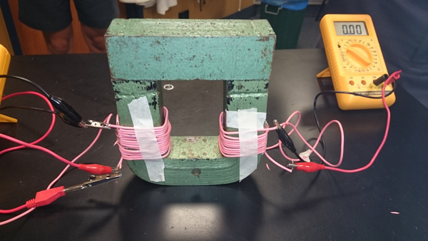
MODIFICATION: Measuring Earth's Magnetic Field Strength with Helmholz Coils
Up until the 1830s it was difficult to measure the magnetic field of the Earth quantitatively because there were no real standard to compare it against. As electromagnetic theory was developed through the 1800s it was found that magnetic field strengths could be given absolute values by the use of a coil carrying an electrical current. In this EEI, you could measure the local magnetic field by comparing it to a know value created by a coil of known size, current, and turns.
If you place a compass on a bench and let it point north, you can make it move towards the east or west by placing a magnetic field at right angles to the compass direction. If you can get the needle to move to 45° it means that the coil's field is the same magnitude as the Earth's field - but just acting at right angles.
You can use the Biot-Savart Law to determine magnetic field strength due to the coil: BC = 8 μoNI/(R x 5√5) where N = number of turns on each coil (not the total), I is the current, R is the radius of the coil. The constant μo is the permeability of free space (4πx10-7 Tm/A).
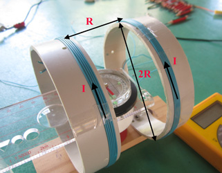
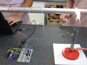
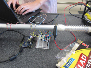
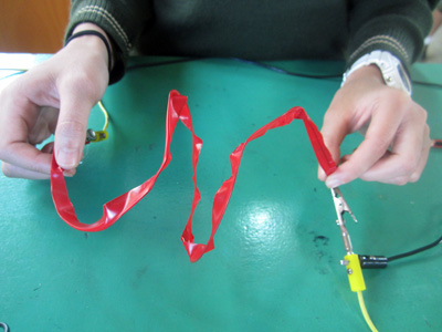
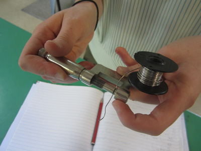
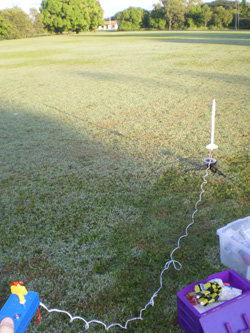
The setup I made was two Helmholz coils with a gap between them for the compass. I placed the compass on a little stand so that it was in the centre of the coils. Plastic water pipe is fine for the coils. I used clear plastic of diameter 109 mm (R = 0.045 m), and wound 25 turns of wire on each one (N = 25). They were orientated so their axis was East-West (at 90° to the compass). I am indebted to Prof. Jon Williams of Bowling Green State University, Ohio, USA, [Physics Teacher V52, April 2014, p252].
 |
 |
Here's my set up looking from above. The distance between the coils should be equal to the radius of the coil. The two coils are connected in series so that the same current passes through both, and in the same direction (as shown). |
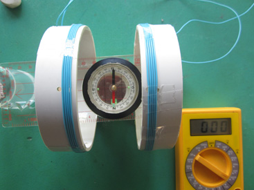
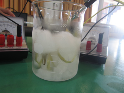
With no charge flowing through the coil (I = 0 mA) the compass reading was 0°. Check that the compass hasn't been stuffed by someone leaving it jumbled up with other compasses and magnets in a drawer. The red end should point North. |
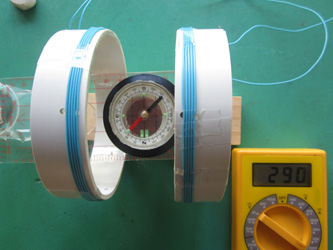
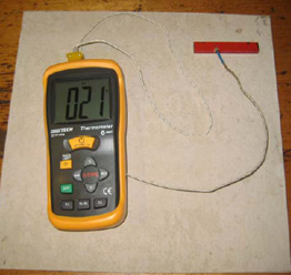
Using a laboratory DC power supply set at 2V connected across a rheostat I was able to vary the current through the coils from 0 to 60 mA. I took compass readings (to the East) as I varied the current, making sure I took a mA reading when the angle was 45°. The photos show some of the readings.
 |
 |
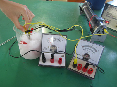
With 290 mA of current the needle had shifted to 45° E. A couple of warnings: the rheostat is a huge source of stray magnetic fields. Keep it and all other steel items away from your compass. The other thing I found was that the digital multimeter and even my camera affected the compass. This experiment was done while I was teaching at Our Lady's Catholic College, Annerley, Brisbane. |
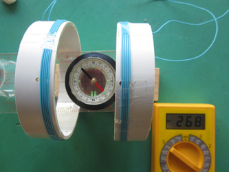
At 268 mA in the reverse direction the needle was deflected to 45° E. Here, the magnetic field strength of the coil equals the horizontal component of the Earth's magnetic field (BC= BH). You can increase the current further: at 132 mA I had the needle at 60° E. I reversed the current and took similar readings for the (negative) angle (to the West). The current registered as negative (-). |
Instead of just using the magnetic field strength value at 45° as a measure of the Earth's magnetic field (horizontal component), you can plot the results to get a more accurate value. The logic is this: at each angular position, the net torque T (tau) on the magnetic compass needle must be zero, if the needle is stationary. Therefore, the torque ΤH due to the horizontal component of Earth's magnetic field and the torque ΤC due to the coil's magnetic field on the needle must be equal and opposite:
TC= TH
μoBCcosΦ = μoBHsinΦ
BC = BHtanΦ
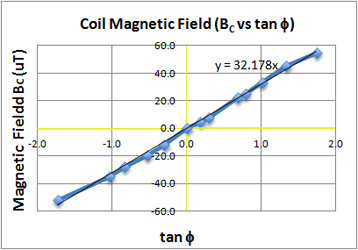
The relationship takes the form y = mx + c. If you plot BC (y-axis) vs tanΦ (x-axis), the graph should go through 0,0 (c = 0) and the slope will be the BH. I obtained a BH of 32.2 μT.
|
| That's a pretty cool graph. The slope is shown by the "y= 32.178x" which means the horizontal component (BH) of the Earth's magnetic field strength was 32.178 μT (microtesla). |
Lastly, once you have BH you can calculate BE (the overall magnetic field strength of the Earth at that location) by dividing by the cos of the local declination angle. The declination angle can be measured by a "dip needle" which should be available in most Science Departments. My measurement of "dip" was 57° South-down (the accepted value for Brisbane is 57.4°). For my BH of 32.2 μT divided by cos 57° I get a BE of 59.7 μT. The actual value from GeoScience Australia for the date and location was 55.154 μT, hence my error was 8% (which is quite large).
This makes an ideal EEI as you can modify your design in an attempt to reduce the error. I'm not sure if I should have made the coil shorter in length by winding the wire over itself - perhaps it would be better but I wanted to be able to count the turns easily.
MODIFICATION: Magnetic Field Strength and Temperature
You may have tried an experiment where you magnetised a nail by rubbing it with a magnet and then when the nail was heated it lost its magnetism. Magnetic Field Strength is affected by temperature. This makes an ideal EEI. In his Year 12 EEI at Villanova College, Coorparoo, Brisbane, student Peter Bergin wrote:"When the magnet is cooled, the borders of the domains slightly move so that the alignment of the domains are further preferential and create a stronger magnet. If the temperature of a magnet is raised, it causes the random thermal motion of the atoms to increase. This motion randomises the domains and the borders are shifted so that they are no longer in a complete single direction like the domains were previous to heating".
He used a Hall Effect field strength probe as shown in the photo below. Peter found a field strength of 45.2 mT at -25°C down to 43.8 mT at 20°C. He suggested liquid nitrogen would be interesting. The EEI may be strengthened by a more direct measurement of the field strength. Rather than a "black box" probe, you could estimate the field by measuring the torque on a compass needle or by the rate of oscillation of another magnet swinging in the field nearby (as they did in the olden days). A comparison of different types of magnets, or length of heating time or different ways of measuring B would be worthwhile.
 |
 |
 |
| Peter Bergin's design | The Hall Effect probe may be better replaced with a less sophisticated device. | Measuring temperature |
MANDATORY PRACTICAL: Conduct an experiment to investigate the force acting on a conductor in a magnetic field.
This is a mandatory experiment in the Queensland physics syllabus (QCAA, 2019). In this experiment a wire is placed between the poles of permanent rare-earth magnets which are lying on the pan of an electronic balance. When electric charge flows through the wire as an electric current there is a force acting upwards on the wire which results in an equal and opposite force downwards on the magnets. This is registered as a scale reading in grams on the balance. The electric current is registered on an ammeter.
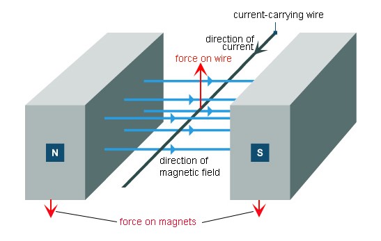 |
| Arrangement of the magnets and current-carrying wire |
The force on a current-carrying wire has been derived as F = BIL sin θ, and the direction of the force has been established by the right hand rule (Figure 1). In this experiment the wire will be at 90° to the magnetic field, and the length will be measured and kept constant. Hence, the relationship is expected to be linear with F ∝ I, providing B, L and θ are kept constant. A graph of F vs I will produce a gradient of B × L. Substituting for L, you will be able to determine the magnetic field strength of the field (assumed uniform) between the poles of the permanent magnets. Analysis of uncertainty will allow you to estimate the magnetic field strength and its percentage uncertainty.
This video that follows below is a demonstration of the force on a current carrying wire in a magnetic field (NCPQ* U3&4 Expt 7.4). I give some hints about how the prac may proceed.
In this video, a strong magnetic field is produced using two 10 mm x 5 mm rare earth disc magnets of surface field strength 0.4667 T (4667 G) held 10 mm apart by a small piece of aluminium channel. A stiff copper wire is held rigidly between the poles of the magnets using a clamp and retort stand. An electric current is passed through the wire and the downwards force on the magnets and channel is shown by a scale reading on the balance in grams. The effective length of the wire in the magnetic field is 10 mm. A series of trials is undertaken with the current being increased from 0.40 A to 1.00 A and the scale reading (converted to Newton, N) goes from 0.0013 N to 0.0033 N. When plotted with current on the horizontal axis and force on the vertical axis, we get a gradient (F/I) equal to 0.0033 N/A. Rearranging the formula F = BIL to B = F/(I L) we substitute 0.010 m for the length (L) and this gives a value for B of 0.33 T. The accepted value for B = 0.4667 T so that means there is a percentage error (E%) = 36%. This seems high but it is reasonable given the limitations of the measuring equipment and the design of the experiment.
I filmed this at Moreton Bay College in November 2018 with the assistance of my very talented student Kayleigh who skipped Chapel to help me. Reference: *New Century Physics for Queensland - Units 3 & 4, 3rd edition, OUP, 2019 by Richard Walding. Chapter 7.4 page 195-200
I made another video (March 2021) showing a close-up of the ammeter and electronic balance so that you can collect your own data if you can't get the equipment to do this practical, or if you've been away from school. It starts with a description of the equipment and forces.
SUGGESTED PRACTICAL: Conduct an experiment to investigate the induced EMF from an AC generator.
MODIFICATION: Transformers and power
losses
Electrical transformers are used to "transform" voltage from one level to
another, usually from a higher voltage to a lower voltage. A changing current in
the first circuit (the primary) creates a changing magnetic field; in turn, this
magnetic field induces a changing voltage in the second circuit (the secondary).
Transformers are some of the most efficient electrical 'machines', with some
large units able to transfer 99.75% of their input power to their output. Your
EEI could be about the factors that influence the power losses. Is it frequency,
voltage, current or just what? What ever you do, don't use mains (240V) voltage.
Use the school's laboratory power pack or a signal generator.
![]()
![]()
 |
Experimental set up by Yr 12 Physics student James Camp at Churchie. (James Camp) |
SUGGESTED PRACTICAL: Conduct an experiment to investigate the induction of an electric current using a magnet and coil.
MODIFICATION: Ring inductance
If you pass an alternating current of about 2000 Hz through a solenoid you can display the waveform on a CRO (I'd adjust the current so that a maximum amplitude is obtained with no noticeable nonlinear distortion; and set the synchronisation at 'external'). Now make up an auxiliary coil from a non-ferrous material such as a piece of aluminium tubing that just fits inside the solenoid. Give it say 6 turns of fine copper wire and place it inside the solenoid.
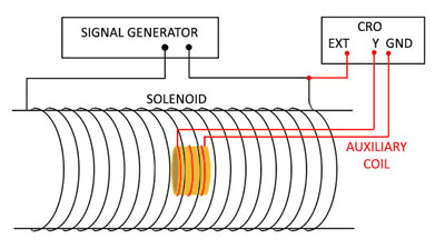 |
By Faraday's law of electromagnetic induction, a current will flow in the ring in such a direction to oppose the changing magnetic flux producing it. Two effects will be observed in the CRO trace. There will be a decrease in amplitude accompanied by a shift in phase. The experiment could be then repeated with other input frequencies (up to 3kHz).
In one experiment I read, for a frequency of 2 kHz the voltage dropped from 4.2V to 3.4V and the phase shifted by 39°. You can use this to calculate the inductance of the auxiliary coil (it was 2.88 x 10⁻⁷ H). There are formulas that you could use to calculate the theoretical inductance and it should be close. For lower frequencies the inductance will be less.
UNIT 1.3 Electricity
Energy output of a solar panel
Photovoltaics (PV) is a method of generating electrical power by converting
solar radiation into direct current electricity using semiconductors that
exhibit the photovoltaic effect. Photovoltaic power generation employs solar
panels comprising a number of cells containing a photovoltaic material. The
Australian Government provides incentives for the use of PVs for both domestic
and industrial use (you can save money, and save the environment). Solar
photovoltaics generates electricity in more than 100 countries and, while yet
comprising a tiny fraction of the 4800 GW total global power-generating capacity
from all sources, is the fastest growing power-generation technology in the
world. Between 2004 and 2009, grid-connected PV capacity increased at an annual
average rate of 60 percent, to some 21 GW.
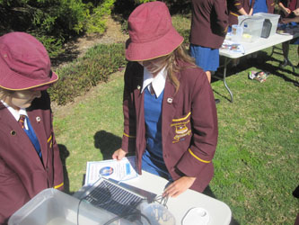
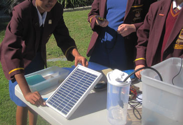
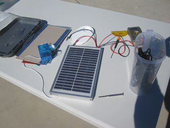
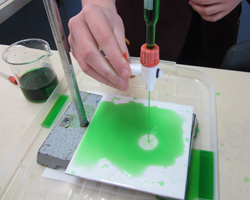
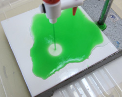
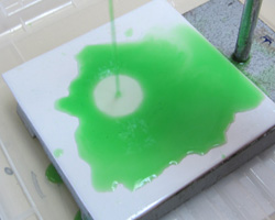
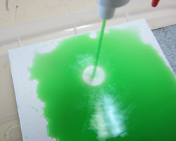
A good EEI would be to measure current as a function of the angle of incidence of sunlight (all within a short period of time eg 30 minutes); measure current when collector is perpendicular to rays during the day (how should that go?). But maybe you'll need to consider more than current; perhaps the power output is more important. If so, you could put a load on the circuit (resistor) and measure V and I. In the method shown below, Moreton Bay College students are measuring the effect of angle on the flow rate (hence power output) of a electrical water pump. This was Year 10.
 |
 |
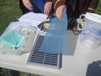
Energy output of a solar panel II
You could also investigate the effect of shade on the output of a panel. In
this photo, students are using layers (1, 2, 3 etc) of shade cloth. It would
also be interesting to see the effect of light of different wavelength to see if
the solar cells are sensitive to all wavelengths. You could use coloured
cellophane - but then that reduces intensity and not all coloured cellophane has
the same percentage transmission. What to do?
The Effect of Dust on Solar Cell Performance
Photovoltaic cells have low conversion
efficiencies (typically up to 20%), the accumulation of sand and dust particles
on their surface further reduces their output efficiency. This limitation makes
photovoltaic cells an unreliable source of power for unattended or remote
devices, such as solar-powered traffic signs or NASA's Mars Rover. For
large-scale solar plants to maintain their maximum efficiency, the photovoltaic
cells must be kept clean, which can be a challenging task in dusty environments.
One good EEI would be to investigate the effect of dust on the solar panel.
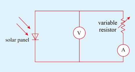
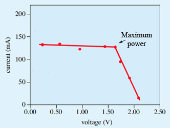
This is a harder EEI than the two above. It involves setting up a solar panel a short distance from an incandescent bulb (eg 15 cm) and adding controlled amounts of "dust" (eg bentonite clay powder, fine sand, icing sugar) to the face of the panel (spread evenly). It is a good idea to adjust the panel so it is working at maximum power. Do this by setting up the circuit on the left below, using either a variable resistor or fixed resistors that can be varied from 0 ohm to 300 ohm. Plot a graph (next figure) to see the maximum power point. Then add the bentonite (0.1g, 0.2 g and so on) and record the V and I (and the product P). Efficiency = Pdust/Pno dust x 100%. A good article is in Physics Education, V45, September 2010, page 456.
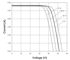
Solar panel output and temperature
The output of a solar photo-voltaic (PV) panel changes during the day for two reasons: one is that the sunlight falling on the panel changes (probably peaks at noon), and as the temperature of the panel rises its efficiency changes. Most panels are rated to put out their maximum power at 25°C, which is a rather unrealistic figure given that the panel temperature under typical Australian conditions can be up to 70°C. Here's what one user (Cabel) said on the Whirlpool Forum:
I have 16 Suntech panels. I don't have the actual voltage outputs vs temperatures, but comparing my best clear day since installation, 19.02 kW max temp 26°C and clear hot day 17.18 kW max temp 41°C. Overall I'm very happy with the reduced output of around 10%. Any cloud cover on these days seems to help output a lot also. I have got 18.5-19 kW on a number of cloudy 40°C days. I also have black tiles but have a good 50mm gap between roof and panels so it should have reasonable airflow. |
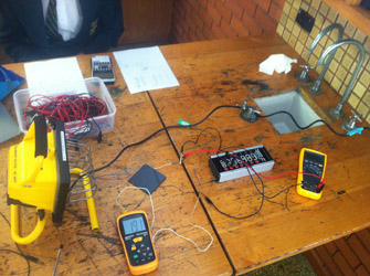
This suggests a good EEI. You could measure the V and I characteristics across a load resistor (say 56Ω) connected to a solar panel. Then with constant illumination, you could put the PV panel on top of a hotplate and crank up the temperature. How high a temperature - well, you can decide. Alternatively, you could hold the temperature constant and vary the illumination. Year 12 student Ryan Phillips from Villanova College, Brisbane, used an electric bar heater in front of the solar panel. The light stayed constant as the panel heated up and he got some interesting results (see setup below).
 |
 |
The power output (VxI) of a PV cell at different temperatures. |
Ryan Phillips' setup at Villanova College. On the left is the bar heater with the Digitec yellow thermometer next to it. In the middle is a resistance box and to the right is a Fluke multimeter. |
 |
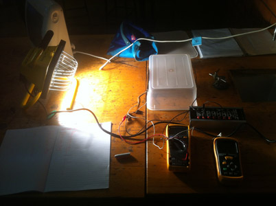 |
Ryan's solar panel illuminated by the heater. |
A side-photo shows Ryan's arrangement. He did very well! |
Thermal Conductivity - Ångström's method revisited
The conductivity of heat through a substance is a significant problem that affects many areas of material science and engineering. How to measure the rate of heat conduction is a big issue. It applies to the design of solar panels, drawing heat from electrical components and even materials used in dentistry. Sometimes they mount semiconductors on diamonds to prevent damage from overheating, since diamonds have an extremely high thermal conductivity.
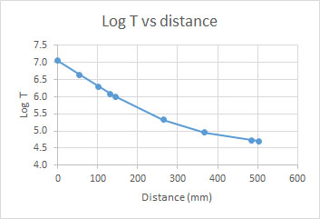
There are many ways to measure conductivity but one that is exceptionally good for a Senior Physics EEI is to use a modified Ångström method. The Swedish physicist Anders Ångström developed this method in 1863. It involves the periodic heating and cooling of a metal rod and measuring the temperatures with sensors along the rod in two positions a known distance apart. You will see the first wave of heat come past the first sensor and a minute or so later it will arrive at the next sensor. A plot of the data is quite revealing.
Below is the plot of such an experiment done by my hero Prof. Alexander Crichton Mitchell in Edinburgh on 9th January 1886. He was measuring the conductivity of ice.
 |
| The time interval between the peaks is 50 seconds and this can be used to determine conductivity [Proc. Royal Soc Ed, V13, January 1886, 592-596]. |
I repeated his experiment using an aluminium rod covered in bubble wrap with sensors held in place with zip ties. For sensors I used LM335Z Temperature Sensor Linear IC (Jaycar $4.50). I used heatsink compound to make sure the sensors made good contact with the rod (compound available from Jaycar $3.95, although I wished I bought the silver based one for $5.95). All you need do is turn your lab hotplate on to 'full', and wait until it is fully hot (the thermostat should click). Place the end of the rod on it for a short time (you decide) and then take it off. You could then place it on some ice. Repeat this in a uniform and periodic fashion.
 |
 |
I used an Arduino to collect data from the two sensors. This time I heated the rod with a Bunsen. If I did it again I would make a shield out of cardboard or foam to stop the convection and radiant heat from getting to the thermistors. My thanks to Nadia and Emerald for helping with this. |
Then I tried wrapping a part of the rod with a plastic oven bag (polyester) and then wrapping a coil of nichrome wire from a jug element around it and connecting it to a 12 V DC supply. That worked but it didn't get very hot so I shortened the wire from 1 m (10 ohms) to about 20 cm and that made it about 2 ohms and about 70W on a 12 V supply. My thanks to Caitlin Ramsay for her help. |
The problem for you is how to display and analyse the data. Sure you can draw a graph that will show the time lag between peaks, and show the size of the peaks. But, if you were doing this for 3rd Year Physics or engineering at uni you'd then do a Fourier analysis to work out harmonics and so on. Far too much for Senior Physics but good to think about. Just Google "Angstrom's Heat Method" or have a look at the method that goes with the Pasco device. I'd be thinking more about comparing different rods (steel, copper etc) and seeing how they compare. The possibilities are huge.
Temperature along a heated metal rod
You are well aware that the closer you are to something hot, the higher the temperature. For instance, if you put the end of a metal bar in a fire the rod will have a high temperature at the red hot end but the temperature will be lower at the other end close to your hand. French scientist Guillaume Amontons (1663-1705), assumed that temperature varied linearly along such the rod but Johann Lambert (1728-1777) found that the temperature profile along the rod declined logarithmically.
He found the relationship to be:
y = 97 + 106 x 5e-x/116.3
 |
| Victoria and Alexa have set up a 12mm diameter aluminium rod on a hotplate. They drilled holes every 10 cm to take thermometers. Moreton Bay College - May 2016. |
 |
 |
To try this out, I took a length of aluminium rod (actually just unscrewed the rod from a retort stand) and stuck LM335Z Temperature Sensor Linear ICs (Jaycar $4.50) to the rod with some heatsink compound (Jaycar $3.95) every 10 cm. These were held in place with wire twisties (zip ties would also work). One end of the rod was placed on a hotplate (150°C) and supported at the other end. I turned it on (about 150°C) and waited until temperature stabilised along the rod. I measured the output of each IC by connecting them in turn to an Arduino with a simple temperature reading 'sketch'. Download my sketch here if you like.
My results were pretty good so I tried it with a much longer rod and got what I think would make a terrific EEI. I guess you could also bore some 8 mm diameter holes in the rod every 10 cm and insert calibrated thermometers. You know that someone will knock it and break one though. Happy times. [Note: to calibrate, just put them all in some boiling water and note the temperatures. Put tape on each one noting how much +/- they are away from 100°C].
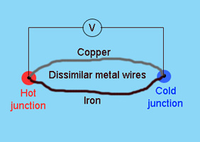
The Thermocouple
One device used widely used in science, industry and medicine to measure
temperature is called a thermocouple. It consists of two wires of two different
materials that are joined at each end. When these two junctions are kept at
different temperatures a small voltage occurs. This voltage drop depends on the
temperature difference between the two junctions. The phenomenon is called Seebeck Effect. The measurement of the voltage drop (or emf) can then be
correlated to this temperature difference. Thermocouples are among the easiest
temperature sensors to use and are very popular because they're generally very
accurate and can operate over a huge range of really hot and cold temperatures.
Since they generate electric currents, they're also useful for making automated
measurements.
Be warned about information you get off the internet about
thermocouples. One popular site says a thermocouple is "...a junction of
dissimilar metals that creates a voltage you can relate to temperature." This
misinformation continues to appear on company web sites, in application notes,
and in articles. You could make a simple thermocouple from copper and iron wire
(see diagram below) using boiling water and icy water to calibrate your device.
Then you could investigate the cooling curve (and time constant) when the hot
end is allowed to cool in a gentle breeze. Or you could look at ways of forming
the junction (twisting, soldering, welding). Or how about different alloys and
what factors influence the voltage (resistivity perhaps). There are lots of
things that would make a great EEI.
 |
 |
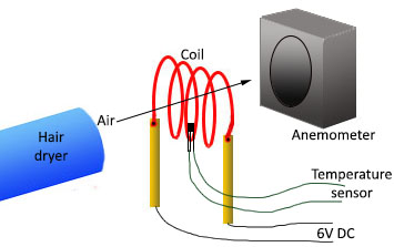
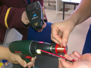
Hot wire anemometry – measuring wind speed
You may have hear of wind chill. When wind blows on a hot object it tends to cool it down, and the faster the wind the greater the cooling. This is the basis of hot wire anemometry. It's a common method for measuring fluid velocity. The technique depends on the heat loss to the surrounding fluid from an electrically heated wire. As the fluid velocity varies, then the heat loss is a measure of that variable. This suggests a great EEI.
If you make a small coil (say 20 cm) of nichrome wire and connect it to a 6V DC power supply it will warm up. Let's say the wire has a resistance of 2 ohm, the power output will be P = V2/R = 36/2 = 18 W. For my test the temperature equilibrated at 40°C. Now when I blew cool air from a hair dryer over it, the coil dropped to a temperature of 31°C. I measured the wind speed with an anemometer to be 1.3 m/s. Higher speeds dropped the reading (eg at 3.3 m/s it was 28°C). I used a digital anaemometer from Jaycar ($70). For temperature I glued an LM335Z Temperature Sensor Linear IC (Jaycar $4.50) to the wire and packed some heatsink compound (Jaycar $3.95, although you may want the silver paste for $5.95).
 |
 |
The setup is pretty simple. You need to glue on a temperature sensor with heat conduction paste. |
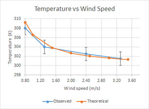
The experimental and theoretical graphs. |
Heat is lost from the wire by conduction to the air, convection in the air and radiation. There is a great paper on this experiment by Prof. Mohamed El Abed Lycée Paul Eluard, Saint-Denis, France in the Journal Physics Education, V51, January 2016. I discussed with Mohamed how this might work as Senior Physics EEI and he gave me some advice (he was once a high school teacher at Lycée Suger in Saint-Denis so he knows what will work).
He eliminated radiation as a possibility as it was so small. The formula Prad = ε σA(Teq – To ) gives a value of 6.49 mW [ε is the total emissivity of the wire (= 0.05 for nickel) and σ = 5.67 x 10⁻⁸ Wm–2 K–4 is the Stephan Constant; A is the surface area of the wire, and T is room temperature in K.
Mohamed settled on a formula based on King's Equation and proposed that Teq = To + RI2/(A + BUeq½ ) [where A and B are constants (-0.275 and +0.575 respectively for his experiments, R = resistance in ohms, and I is current in ampere]. It is very difficult to find the equation for the (non-linear) curve so for Senior Physics, you may not wish to do so. However, don't let me stop you trying. But as Mohamed said "...fair agreement with King's law gives consistency to the measurements; the purpose is achieved: students realize that they are able to re-discover a known physical law. Further qualitative discussions about the validity of the law and the accuracy of the measure are then welcome. Since we are dealing with non-linear fitting, you will always be able to find a set of parameters that fits the curve but that has no physical ground."
There is plenty of room to discuss errors though, and how they can be addressed. The mathematical formula gives the curve that best fits the experimental data within the error bars. But it is to be used with caution: The existence of a cut-off speed U greater than 0.228 ms-1 has a physical interpretation. It means that it's not possible to reach U = 0 ms-1 with this method. Mohamed pointed out that:
"When the speed is zero (which is always the case on the boundary layer of the wire), the heat flux is due to conduction only; this means that the Nusselt number (Nu) is equal to 1. Since measurements are performed far from the boundary layer, the measured speed is never equal to zero. The mere existence of an equilibrium temperature Teq above room temperature is related to the existence of a flow. Since Teq– To is at most equal to a temperature rise of 55K, Nu (proportional to 1/( Teq– To) is at least equal to 20. This means that in the conditions of the experiment, U can never be equal to zero and conduction heat transfer can be neglected. King's Law is an empirical law only valid for a cylindrical wire in an incompressible low Reynolds number flow. It depends on many hidden parameters like the aspect ratio, the orientation of wire with respect to the flow, the presence of a solid surface nearby that would be responsible for an increase in heat transfer, turbulence, the Prandl number. This might explain why the model fails at low speeds. Very often in fluid mechanics, no analytical solutions are available since many dimensionless numbers are inextricably linked and very often, experimental data (obtained with calibrated sensors in flows of known speed) are used to determine the coefficients that relate these dimensionless numbers between them. |
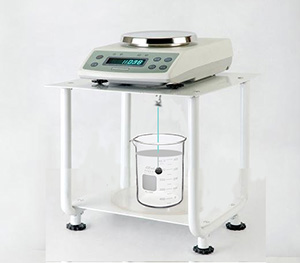
Density of water at different temperatures
Senior Lecturer in Physics, Stephen Hughes, from Queensland University of Technology, described a technique for measuring the density of water at different temperatures. It applies Archimedes' principle to investigate the effect of global warming on the oceans, namely that a large component of sea level rise is due to the increase in the volume of water due to the decrease in water density with increasing temperature.
It is a simple technique: water close to 0°C is placed in a beaker and a glass marble hung in the water from the underside hook of an electronic balance. As the water is warmed (perhaps hotplate and bar stirrer), the scale reading on the balance increases with temperature as the water is less buoyant due to the decrease in density. Once the temperature reaches say 50°C, you could let it cool and take a second set of readings. Stephen used a balance with a precision of 0.1 mg and a marble of volume 40.0 cm3 and mass of 99.3 g, yielding water density measurements with an average error of 0.008 ± 0.011%.
 |
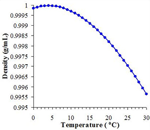 |
| Setup for measuring the density of water. The scale reading on the balance allows you to calculate the upthrust. You need to know the volume of the marble accurately. | Typical graph. How well do your data agree with this graph. What are the sources of error? |
A good EEI could be made out of this by looking at the sources of error when a graph of results is compared to known results. Further investigations could be to try water of say 1%, 2% and 3% salinity at various temperatures. See: Stephen Hughes and Darren Pearce "Investigating sea level rise due to global warming in the teaching laboratory using Archimedes' principle", European Journal of Physics, Vol. 36, No. 6, September 2015.
Temperature and Resistance using nichrome wire - Part 1
Here's an extract from my textbook about resistivity and temperature:
Like many physical properties, resistivity not only depends on the material involved but also on the temperature. The resistivity of pure metals increases linearly with temperature because a temperature increase causes the lattice ions to vibrate with greater amplitude. This increases the likelihood of electron collisions and decreases the current through the conductor. The expression for the increase in resistivity with temperature for any conductor is: |
This can make a good EEI despite the relationship being so well known. As mentioned above, nichrome has a fairly high resistance (typically 10 ohm/m). The problem with changing the temperature of the wire is that if you use a water bath you may have to wind the wire on to a spool so that it doesn't short circuit on itself. Another way is to insulate the wire is with electrical tape or masking tape. That's what the girls at Our Lady's College, Annerley, did:
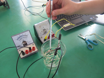 |
 |
The nichrome wire is covered with masking tape so it can't short circuit. Eloise's hand - at Our Lady's College. |
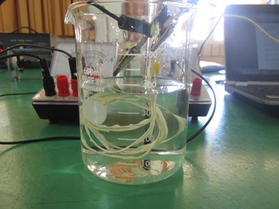
Close-up of the wire in the beaker at room temperature. They tried it in liquid nitrogen at -196 °C (thanks to Griffith University), dry-ice at -78°C and boiling water as well. |
The other problem is that if you measure the resistance by impressing a volatge across the wire and measuring the current, you will get Joule heating. You will need to be careful about what voltage you use (and perhaps try a few to see what effect it is having). Great source of errors for discussion. You could also twist the wire into a loose coil (without the turns touching) to see if there is an interference from one turn on the next.
 |
 |
Lyly holds the the wire that she wrapped in electrical tape (Our Lady's College - May 2014). |
You should measure the diameter with a micrometer at right angles to each other to make sure the wire has a circular cross-section (and is not oval). You should also measure it at several places along the wire in case it has been stretched in parts. It wasn't. |
 |
 |
In Dry Ice at a temperature of -78°C. |
Probably better to use the 50mA scale to get a more accurate reading. |
Because the change in resistance is not large you need to choose your meters and scales with care. A 2.5 m length of nichrome wire may be 25Ω. If you have a voltmeter that has a full scale deflection (FSD) of 1V then the wire should give a current of about 40mA. This will fit nicely on an ammeter with a FSD of 50mA. In the photo above the girls have chose to use the FSD of 500mA range as their current was 55mA and just off the 50mA scale. It is all a balance of wire length and voltage so that the readings are close to FSD.
Temperature and the resistance of nichrome wire - Part II
As mentioned above resistance in wires is difficult to measure accurately because most metal resistance is too low to accurately measure by standard means (ammeter and voltmeter). It should be possible to do it accurately with a Wheatstone Bridge, but if using wire with low resistance (eg copper, aluminium, steel) you may find issues with the resistance of connectors being significant. However, using something like nichrome should work OK. A jug element is a simple way to experiment with nichrome.
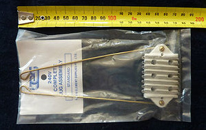 |
 |
Jug replacement kits are available from K-Mart and hardware stores for about $20. The resistance at room temperature is about 37Ω. |
Close up of the jug element: nichrome wire with a diameter of 0.30 mm (28AWG). |
Jug elements - like most water heating elements - use Nichrome 80/20 (80% nickel, 20% chromium). Students' results show that the element is made of 0.3 mm nichrome wire, and if the temperature change is 100°C, the hot resistance of 38.2Ω is about 1.2Ω higher than when at room temperature. In an EEI you would have to look at resistivity, temperature coefficients of resistance and why - at an atomic level - resistance changes. The bigger the temperature change the better. Under teacher supervision you could try really cold things like liquid nitrogen (-198°C) or dry ice (-78.2°) and hot things like heated cooking oil (canola oil has a smoke point of 204°C, but do with teacher supervision).
Physics Co-ordinator Peter Finch from St Joseph's College, Gregory Terrace, Brisbane, said that the results from such experiments are generally excellent (if the experiment is done properly). He makes this suggestion:
There is one possible downside and that is the measurement of resistance. Since resistances are very small, I hire two microohmmeters - from memory these cost around $300 per week. If you do the preparation properly, you could get away with one microohmeter for a week if you have say 40 students, but be prepared to work before school and at lunch. For my eighty [Year 12] students (a good number will do the resistance EEI) I use two microohmmeters for two weeks. The apparatus costs roughly $5000 to buy.
There is an alternative to the microohmmeter and that is a set up using a Wheatstone Bridge. The circuit is very simple and costs roughly $30 from memory (this includes $20 for a multimeter). I did a comparison with the Wheatstone Bridge and the microohmmeter and found remarkable accuracy over a wide range of resistances. From memory it was not particularly accurate over the lower range of (say) 1 to 1500 microohms. You can get around this issue by using longer and/or thinner wire.
Temperature and the resistance of wire - Part III
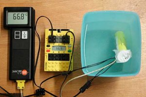
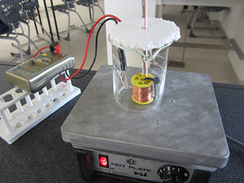
One other way to get a reasonable resistance change from copper wire is to use a long length of it. Three of my Year 12 Physics girls (Georgia, Shannon and Georgina) at Moreton Bay College made up coils of copper wire on cotton-reels in an experiment about guitar pickups. In one case they wound a coil of 800 turns of 0.25 mm diameter enamelled copper 'armature' wire. When they had finished I used it for an experiment on resistance and temperature (see below). They didn't know I took it but it works well.
 |
Here they are winding the coils for the guitar pickup EEI. See details further down. |
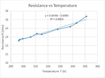
I connected it to a multimeter set to measure resistance. At room temperature it was about 13 Ω. I placed it in a beaker on a hotplate, with a lid of polystyrene, and added a thermometer through the middle of the spool. I heated it to 70°C, measured the resistance (about 16 Ω) and turned the hotplate off and let it slowly cool. Over the next 30 minutes it dropped back to room temperature and as it did so I took measurement readings. Here's my setup and graph. The girls didn't see me do it as they were busy writing up their EEIs; well some were - the rest were complaining about having five assignments to do over the holidays. The graph pretty-much passes through 0Ω at 0K, and the temperature coefficient of resistance is pretty close to the accepted value. I know this could be greatly improved - but it seems to work.
 |
 |
My 65m coil of wire being warmed up. |
My graph. Pretty rough - but I'm only doing it for fun. [16 June 2015] |
Storing charge in a home-made capacitor
Capacitors are quite simple things really: two sheets of metal foil separated by a thin sheet of paper or plastic. They are used to store electric charge. However, they are absolutely fundamental to most electrical devices from mobile phones, radios, motors, computers and so on. Their properties have been known for a few hundred years but new developments happen all the time. For instance 18 year old Eesha Khare of California developed a supercapacitor that can recharge a mobile phone battery in less than a minute. She won the Intel Foundation Young Scientist Award of $50,000 and has been approached by Google.
The relationship between capacitance and plate separation for a parallel plate capacitor is well known: C = κ εoA/d which shows that capacitance is inversely proportional to separation distance (d). Typically, the dielectric thickness is varied by using increasing numbers of sheets of paper or plastic (whatever dielectric materal you choose). But when you examine the results you often find that the inverse relationship (C ∝ 1/d) doesn't hold too well. It seems that the air between the sheets confounds matters. This suggests a great EEI.
Measure the capacitance of a home-made capacitor using a digital multimeter (with capacitative measurement) and vary the number of sheets of dielectric. These multimeters are cheap ($15) but you may need to buy one in). Then repeat but try increasing the pressure on the plates by adding increasing weight (brass masses or house bricks) and see what that does. Physicists at Indiana University (USA) did just this and found some interesting and unexpected trends (American Journal of Physics, V73 (1) Jan 2005, 52-56).
 |
 |
 |
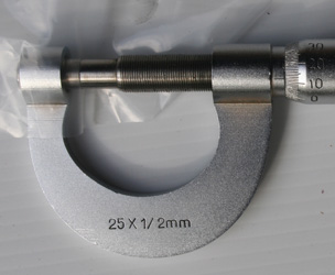
The sheet thickness can be measured with a micrometer. In the photo above, a reading of "12" on the thimble and "0" on the barrel gives a thickness of 12/100 x 0.50 mm = 0.060 mm. This is because 100 divisions on the thimble is equal to 1/2 mm on the barrel (as shown by the marking "25 x 1/2 mm" on the frame. Not easy for students to appreciate. |
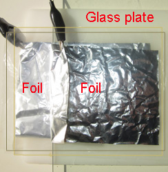
I laid the foil on a plastic cutting board to raise it a bit so the alligator clips could be attached, and then made a sandwich of foil, two sheets of plastic dielectric, the top foil and a sheet of thick glass on top. The dielectric is outlined as two rectangles in the image so you can see the edges. The glass is not easily visible but I used glass so you could see the insides of the setup. |
Then I added a 1.5kg "weight" (15 N) and remeasured the capacitance. Then two weights and so on. You need something rigid for the weights to press on. I used glass so you could see inside but something like a thick piece of wood maybe better. |
Here's the clever part. Instead of just using multiple layers of plastic as the dielectric, what you could do is buy various thicknesses of the same sort of plastic. For instance, you can get clear "Centrefold" builder's plastic in thicknesses of 50μm, 100μm, and 150μm. That way there is no air gap and you may be able to show that the results are more like you'd expect and what this means about the idea that air is an issue.
Capacitors and heating water
If you are into electricity and want a bit of danger, this EEI may be for you. It looks at the energy stored in a capacitor being released to heat water. Will it be 100% efficient is the question.
Capacitors can store charge so they can be a source of electrical energy. This energy may be released slowly or quickly depending on the resistance of the load. Care must be taken when touching capacitors because you can't tell if they are charged simply by looking at them. Although they may be disconnected from a supply they may still retain a charge, and this stored energy can give you a serious shock! This happened to me when I was taking apart a camera flash.
 |
 |
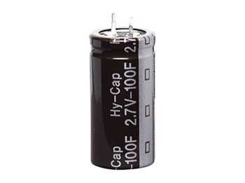
Example of a suitable capacitor: 220 Farad, 2.7 V. When you charge it you will need a resistor to ensure the current doesn't go over 3.56A as stated in the data table for this device. Also, make sure you doesn't exceed 2.3 V. I got this one from Altronics, Brisbane for $22.95. Click here for the catalogue entry. |
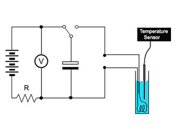
This circuit is a good starting place for your EEI. The battery or power supply used to charge the capacitor should not exceed its rated value (eg 2.7V in the one to the left). The current should also not exceed the rated value (in this case 3.56A). |
The energy stored in a capacitor is given by W = ½ CV2 and the amount of energy absorbed by the water is mcΔT. Set up the circuit shown below and charge the capacitor by connecting it across a battery. You will need to work out how to do this. As the capacitor charges up, the potential difference across its plates slowly increases and the time taken for the charge on the capacitor to reach 63% of its maximum possible voltage is known as one time constant, (Τ, tau). It is equal to the product of R and C where, R is in ohm (Ω) and C in Farad (F). It takes a time of 5T to fully charge the capacitor. So, charge up the capacitor for 5Τ and then switch it to discharge through a small coil in some water. You could experiment with the heating coil but a short length of nichrome wire may work. Keep the volume of water small so the temperature rise is reasonable. Just watch out for the heat losses into the wire, the container, the air and the sensor.
One question is what is a suitable size for the capacitor. You need enough energy stored in it so you can get a reasonable temperature change in the water. A 220F 2.7V capacitor fully charged has W = ½ CV2 = ½ x 220 x (2.7)2 = 800 J. If all of this goes into heating say 25 mL water, you can use Q = mcΔT to calculate ΔT, which would be = 800/(0.025 x 4180) = 7.6°C. That is reasonable if your temperature sensor is accurate enough. You can get higher voltage capacitors (eg 32V) but you have to wonder how you'd charge them in the lab (with a lot of batteries in series). Remember that the stored charge can be quite high and dangerous. Talk to your teacher before you do any trials, and don't hack open an old TV to get the capacitor out as it could still carry a lethal charge.
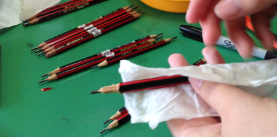
Voltage and resistance of graphite
Whereas the voltage/current relationship for metallic conductors is esentially linear, this may not be so for non-metallic conductors. An excellent EEI can be done on graphite pencil "leads". They are not really lead (Pb) metal but a mixture of powdered graphite and clay. They do come in different hardnesses and diameters, but they are brittle so it is sometimes problematic getting a good electrical connection. Physics teacher Alan Whyborn at Urangan State High School, Queensland, makes this suggestion for an EEI: "You can qualitatively examine the effect of temperature by collecting a set of readings in the air at different voltages (V being the independent variable). But note, the leads will get red hot. You could collecting another set of readings under water." This looks like a lot of fun - probably too much fun. If you get a negative temperature coefficient (opposite to metals) then start thinking that perhaps the thermal energy of the electrons is enough to put more electrons into a conduction band. Over to you.
 |
 |
Two pencil leads: each 0.7 mm diameter and 1.3 Ω resistance with no charge flowing. (Bill Rentschler) |
When 15V AC is impressed across the ends a current of 1A ensues and they get very hot (Joule heating). (Bill Rentschler) |
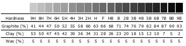
Resistance of different types of graphite
Carbon composition resistors are made from a molded carbon powder that has been
mixed with a phenolic (or wax) binder to create a uniform resistive body. It is then
surrounded in a insulating case after attaching end leads. The greater the %
carbon the lower the resistance. You could model a resistor using graphite
'lead' pencils. The table below sets ou the composition of the various types of pencils:
 |
 |
 |
| These are the 16cm long pencils being used. At this length the "Joule" heating effect is not strong but they kept them cool by wrapping them in wet tissues. | A 16cm long 6B pencil gave a current of 2.25mA when 6.0V DC was impressed across its ends. If you measure the diameter you can calculate resistivity (45.0 Ω.m). |
For an EEI you could measure the resistance (V vs I) for 6B through to 2H pencil graphites using
% graphite as the independent variable. If they heat up then you will have to control the temperature variable but perhaps you could do that by immersing the "leads" in water. My students Jess and Jamie from Our Lady's College got some terrific results for their EEI. For each type of pencil they used three different lengths as well so they could check if R was proportional to L (to eliminate that as an artefact of the experiment). I won't give away all of their results but for 2B and 4B pencils they obtained resistances of 4.01 and 2.55 Ω respectively (ie a resistivity of 95.35 and 98.26 Ω.m). The Queensland Curriculum and Assessment Authority has a sample EEI on pencil leads that you may find useful. It is an "A" level and shows you what a teacher would look for at this level. Click here to download (pdf).
Resistivity of Play-Doh
Here's a good EEI if you like playing with Play Doh and want to investigate the properties of ohmic materials and resistivity while having fun. Play-Doh is a modelling compound used by young children for art and craft projects at home and in school. It was first manufactured in Cincinnati, Ohio, U.S. as a wallpaper cleaner. It is composed of water, a starch-based binder, a retrogradation inhibitor, salt (NaCl), lubricant, surfactant, preservative, hardener, humectant, fragrance, and color. A petroleum additive gives the compound a smooth feel, and borax prevents mold from developing.
Applying a voltage difference across a conductor and measuring the current flowing through a resistor allows the resistance of the conducting material to be determined. From this you can calculate the resistivity if you know the length of the sample and its cross-sectional area. From work done by Christopher Fuse and colleagues at Rollins College, Florida, USA, Play Doh is ohmic up to about 1 V (thanks to the sodium chloride) and thereafter non-ohmic[The Physics Teacher, V51(6) Sept 2013, pp 351].
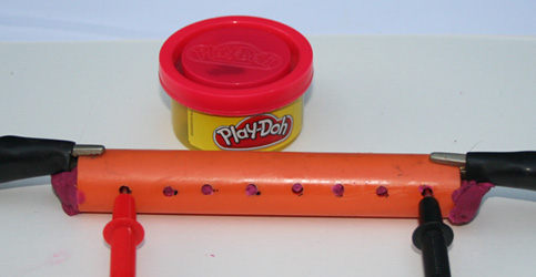 |
Plastic conduit filled with purple Play Doh. A big thank you to my grand-daughter for the use of her Play Doh. It was returned undamaged. |
A good method would be to get a plastic tube (eg electrical conduit) and drill a few holes in the side. Then fill it with Play Doh and poke electrodes in the ends. As the V and I are increased, you can measure the voltage drop across two voltmeter probes placed at a measured separation in the Play Doh. I tried an external voltages from 0.1V to 1.0V and measured voltages between the probes at different distances. I found resistivities of about 0.2 Ωm. You could investigate the conditions (and reason) under which it becomes non-ohmic. If you want to see how the resistivity changes over the day, the ends need to be sealed with cling-wrap or something else to stop it drying out (and resisting the movement of charge). You may like to try different diameters of pipes as well. It all goes towards seeing if the measurement of resistivity of this funny stuff is subject to different lengths, areas and voltages. Chris Fuse said about the time factor:
| All colors of Play Doh have resistivities that vary as the natural logarithm of time. Only the red Play-Doh experiences a significant change in resistivity, increasing by 0.06 Ωm. We are unsure of the cause for the red Play-Doh's extreme resistivity change. |
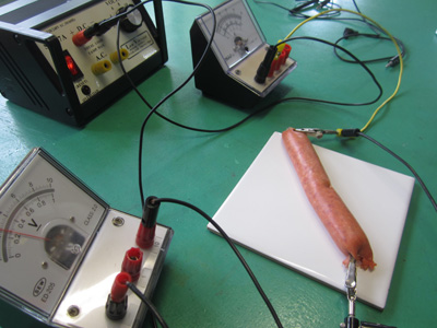
Resistance and temperature for non-ohmic sausages
You can cook food by forcing an electrical current through it. This method of cooking is known as ohmic heating and was proposed at the end of the 19th century. However, no clear conclusion has been reached with regard to the potential use of ohmic cooking in commercial meat processing.
The suitability of food for ohmic heating is essentially dependent on its electrical conductivity and there are critical values below 0.01 S/m and above 10 S/m where ohmic cooking is not applicable because of the large currents needed to get the Joule heating effect. There is little information about how the conductivity of processed meats changes with increasing temperature but what information there is seems to indicate that it increases [Palaniappan & Sastry, 1991]. Secondly, knowledge of the electrical conductivity of meat may give important knowledge about electrical safety for humans. In this regard, determination of the electrical conductivity of a sausage maybe a worthwhile investigation.
 |
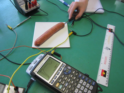 |
Setup used by Year 12 Physics students Morgan and Paris at Our Lady's College, Annerley, Brisbane, for testing a beef BBQ sausage. It was a bit smelly on day 2. |
Morgan and Paris used a Vernier temperature probe connected to a Texas CBL-2 and it worked well - but any similar interface would be fine. |
There are many problems with this though. Firstly, you may wish to know if the sausage is an ohmic resistor - by increasing V across its ends and noting the current through it. But herein lies the problem: as you increase V the sausage will warm up due to Joule heating and its resistance will thus change. You have to keep temperature constant for Ohm's Law to be checked. That's your first problem.
 |
Ohmic Cooking of Processed Meats and its Effects on Product Quality. G. Piette, Journal of Food Science, V 69 (2), pp71-78, March 2004. |
Secondly, you could make use of Joule heating to warm up the sausage and then measure its resistance (V/I) as it warms. This would enable you to calculate conductivity (1/R) as a function of temperature. At each chosen temperature you could also calculate its resistivity and work out the change in resistivity with temperature (knowing the length and diameter would be necessary). If you are tempted to eat the sausage when you have finished - don't. The bacteria may have had a field-day while the sausage is left warm.
*Palaniappan S, Sastry S K. 1991. Electrical conductivity of selected juices: influences of temperature, solids content, applied voltage, and particle size. Journal of Food Processing and Engineering 14:247-60.
UNIT 3 GRAVITY & MOTION
PROJECTILES
NOTE about projectiles & weapons:
|
|---|
A potato gun is a "firearm". |
The potato cannon (or "spud gun") shown on the left is likely to be a Category B weapon as it is a "Muzzle Loading Firearm". It is classified as a "firearm" as it is a "weapon that on being aimed at a target can cause death or injury". "Injury" is defined as "bodily harm" which is further defined as "causing a bruise". If it is a weapon then you may need a firearms license to operate it. A small "spud" (potato) gun may or may not be a firearm depending on whether it can cause a bruise. You should check and not rely on any of the comments above. This category is likely to be clarified in the second phase of the Weapons Amendment Act legislation (after the 2012 State Government elections on March 24). The first phase of the Amendment Act 2011 become effective on 2 January 2101 and 2 April 2012.
Catapults, trebuchets, and bows & arrows - are not considered weapons (even though they can be lethal). If they are used for a "behavioural offence" to harm someone (eg attack them) they then become a "weapon" under the Act and the rules about bodily harm apply. This is similar situation to a baseball bat, a kitchen knife and so on which are also not weapons unless used for a behavioural offence. Catapults, trebuchets & bows & arrows fall in to this area. If a projectile from your trebuchet goes off course and hits someone on the head 100 m away and causes bodily harm then you or the school may be a big legal and medical problem; but it would appear that the police would not consider it an offence under the Weapons Act as it is not a "weapon" and a "behavioural offence" was not intended despite bodily harm being done. Someone may get sued, lose their job, or whatever, but not for a breach of the Weapons Act. Further, none of the above should be taken as a legal advice as it is merely my understanding based on a conversation with officers from the Queensland Weapons Licensing Branch.
Risk Assessment
Teachers in non-government schools may find the Queensland Department of Education, Training and Employment's Curriculum Activity Risk Management Guidelines (CARA) useful.
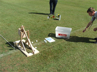
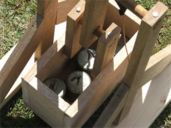
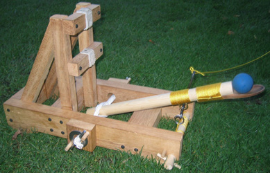
Making and testing a
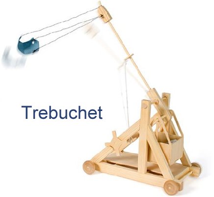
catapult - the trebuchet
A catapult is any kind of device that shoots or launches a projectile by mechanical means. There are many types of catapult. Today 'catapult' describes any machine that hurls a projectile, and one example is the trebuchet. A trebuchet is a siege engine that was employed in the Middle Ages either to
smash masonry walls or to throw projectiles over them. It works by
using the mechanical principle of leverage to propel a stone or other projectile
much farther and more accurately than other catapults. The sling and the arm swing up to the vertical position, where usually
assisted by a hook, one end of the sling releases, propelling the projectile
towards the target with great force. The projectile force of the trebuchet is obtained from the gravitational potential energy of a heavy weight. Among the various types of catapult, the trebuchet was the most accurate and among the most efficient in terms of transferring the stored energy to the projectile. You could investigate the variables to
optimise a catapult/trebuchet (see photo below) - measure range vs. GPE of
weight, length and position of arms; why do these affect range?
Please note:
it is all very well to make spectacular and intricate trebuchets (eg carved and
polished oak or pouring your own lead counterweight complete with ancient
inscriptions of battles won), and it is all very well to do heaps of testing
(battling each others castles on the footy oval); but unless you meet the
requirements of the criteria in analysis, discussion, evaluation etc there is
little hope for a good EEI grade. Be warned! Your teacher will also be
concerned about safety (see "weapons"
note above). You will have to get parental supervision if you are
using power tools or testing it at home. Secondly your teacher will no doubt
place a limit on the size of the throwing arm/counterweight or the projectile.
Some teachers have wisely said: the trebuchet must be small enough to fit on a
school desk; the projectile should be soft, eg a softball; or the projectile
should have a mass no more than a golf ball. Teachers report
some lethal trebuchets used to launched huge projectiles in the back yards of
suburbia. However, there have been students who made ballista (ie catapults) out of paddle-pop
sticks and received an "A".
 |
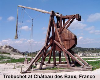 |
| Home made trebuchet - okay for an EEI | Not okay! |
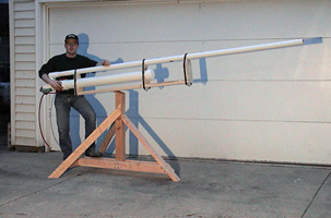
Below are some photos of the setup Luke Hoffman
from Carmel College, Thornlands, used for his trebuchet EEI in Year 12.
Extra photos can be downloaded (click here).
 |
 |
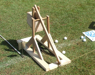 |
| Luke Hoffman sets up his trebuchet on the oval at Carmel College. | The counterweights | Close-up of the trebuchet |
Making and testing a
catapult - the mangonel
A 'mangonel' is another form of catapult that relies on potential energy to provide the projecting force. It consists of a long, wooden arm and a bucket (medieval models used a sling) with a rope attached to the end. The arm is then pulled back (fromthe vertical). Elastic potential energy is stored in the tension of the rope and the arm. A mangonel does not release its energy in a linear fashion. The arm makes an arc (portion of a circle) with a radius equal to the arm's length. Therefore, the potential energy is transferred into rotational kinetic energy and to translational kinetic energy of the projectile. The difficult question before you even start is: what will be your independent variable and how will you measure it?
 |
Home-made mangonel. The twisted rope in the middle of the base stores the elastic potential energy. |
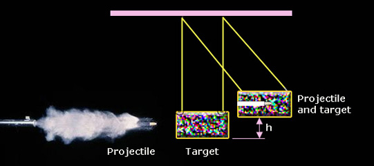
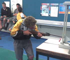
Ballistic pendulum - speeds of projectiles
The motion of projectiles - balls, bullets and arrows - always makes a popular EEI. One of the things you may need to measure is the speed of the projectile and this can be tricky. An old-fashioned way is to use a device called a ballistic pendulum (see below). It was invented in 1742 by English mathematician Benjamin Robins to provide the first way to accurately measure the velocity of a bullet.
Once, students would do this prac using live ammunition. They would fire their guns at a wooden block suspended by a rope (i.e., a simple pendulum). By measuring how high the pendulum swung, they could determine the initial velocity of the bullet. Robins' original work used a heavy iron pendulum, faced with wood, to catch the bullet. Today, in university physics labs through the world they have these elaborate and costly devices for students to us. However, the physics principles tend to get lost in the bells and whistles.
 |
 |
The momentum of the projectile is transferred to the stationery target. The kinetic energy of the target is conserved as gravitational potential energy. |
Year 12 Physics students at New Plymouth Boys' High School, NZ |
I used to use an air-rifle and fire pellets into a small ball of clay. But you can't do this today in class as it is too dangerous. But you could do it with a bow and arrow, or a ball launched from a small catapult and so on. There are plenty of explanations on the internet about the type of collision (elastic/inelastic) and whether momentum and/or mechanical energy is conserved. The maths is not too complex but making the apparatus work without errors is the challenge.
The simplest ballistic pendulum is just a absorbent target (clay, plasticine, toilet roll, foam) hanging on a single string. Robins used a length of cotton thread to measure the travel of the pendulum. The pendulum would draw out a length of thread equal to the chord of pendulum's travel. Great idea that still works well. But if the target rotates at all when struck then some of the translational kinetic energy is transferred to rotational kinetic energy and not to gravitational potential energy. How do you stop this?
So where is the EEI in this if it is so simple? The aim is not simply to measure the velocity of a projectile (ho hum) - but it could be about extending or refining this idea. That's what turns a "cook-book" prac into an EEI. You could compare this method with some other method for measuring projectile speed (time-of-flight, range); you could look at how the accuracy varies with the relative or absolute mass of the projectile and target, or its speed; or the angle through which the pendulum swings. You could look at whether four strings better than two or one; is any kinetic energy converted to heat; does the period of oscillation of the pendulum bear any relationship to the velocity (it does, but how)? This could be quite a remarkable EEI.
UNIT 2.1 - Linear Motion and Forces
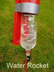
Optimise a water rocket
A water rocket is a type of model rocket using water as its reaction mass. The
pressure vessel - the engine of the rocket - is usually a used plastic soft
drink bottle. The water is forced out by a pressurized gas, typically compressed
air. As the water is ejected the rocket's mass becomes less so less force is
needed to maintain acceleration; but as the gas expands it's pressure becomes
less and can provide less force. How do these competing factors affect the
motion of the rocket. You could look at height or time of flight vs initial mass
of water, pressure, nozzle area, mass of rocket. Explain the physics to justify
your hypothesis or will you do it by trial-and-error?
 |
 |
A detailed examination of
the maths behind water rockets has been provided by Dr Peter Nielsen from
Department of Civil Engineering at the University of Queensland. Click here to
download. He has also provided a rocket simulator spreadsheet to examine the
factors theoretically.
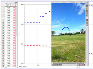 |
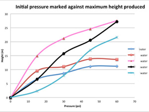 |
Data analysis of rocket flight video using Logger Pro - by Georgia W at Moreton Bay College for her Year 12 EEI. |
Georgia W's graphs of maximum height vs pressure at different water volumes. Whoa - that looks interesting. |
Factors affecting the trajectory of a solid fuel rocket
This is a popular one if you are able to get hold
of rocket "motors". At Home Hill SHS, Queensland, Yr 11 Physics
students undertake EEIs based around rocket flight with their Physics teacher
(and resident Rocketman) Mr Robert Scalia. Here's a part of the introduction
student Patrick Puddlefoot from
Home Hill SHS, Queensland wrote in his EEI: A rocket has four basic
forces acting on it when in flight. These forces are lift, weight, thrust and
drag. The lift force acting on a rocket in flight is usually pretty small. The
other three forces, however, all directly impact the maximum height the rocket
can reach. Weight is a function of how each component of the rocket is
designed. The lighter the rocket is, the higher it will be able to go all else
being equal. Thrust is generated by the rocket's motor. The more thrust the
motor produces, the higher it will go. However, neither of these forces is
heavily dependent on the nose shape. The force that has the most effect and does
vary significantly with the shape of the nose is drag.
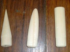
Patrick decided to investigate nose shape (cylindrical, elliptical and pointed) as a factor in a rocket's performance. You can read his abstract here along with a couple of his data tables and a comment on the method. The rockets and altimeters were purchased directly by Robert Scalia from ApogeeComponents in the USA. He said there were no real problems apart from some faulty launch controllers "which they replaced promptly". Rockets are quite inexpensive and the altimeters cost approximately $90 each (but are reusable). "Estes" C6-5 engines were purchased from the local Toyworld store for $14.99 for a pack of 3. Click here to see the Toyworld catalogue page. Robert said that he was looking at less powerfulengines in 2011: "The C6-5s are spectacular but you need a large area for testingand a small amount of wind as it's likely they will go missing". Note: The letter "C" represents the total impulse in newton seconds: A = 2.5, B = 5, C = 10, and D = 20. The first number after the letter represents the number of seconds of engine thrust. The second number represents the number of seconds of delay between the end of engine thrust and the reverse (recovery system deployment or second stage ignition) charge. Thus a type C6-5 delivers 10 newton seconds of thrust in a six second burn, followed by a five second delay. Other common types available are: A8-3, B4-4, B6-4, B6-6, C6-3, C6-5, C6-7 and (gulp!) the D12-5. I'm guessing Home Hill SHS will be going for the B6-4 this year.
 |
 |
 |
| Patrick's nosecones. Extra mass was added to the payload of the pointed and elliptical cones so that each rocket had the same mass. | The altimeter: once the rocket was back on ground the altimeter will be heard to make an irregular beeping sound. These beeps tell you how high (apogee) the rocket reached; e.g. five beeps followed by two beeps followed by two beeps means that that rocket reached an apogee of 522 ft. | The altimeter's data can be downloaded via a USB connection and analysed for altitude, acceleration and velocity of rocket flight. More photos from Patrick's EEI can be seen here. |
The photos below were taken by Amanda and supplied
by Physics teacher from Home Hill SHS - Mr Robert Scalia.
 |
 |
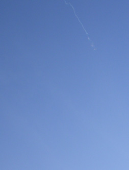 |
| Megan Lipsys and Paul Barker measure the characteristics of different nose cones using a TI Ranger, and a TI CBL2 data collector. | Detonating the rocket engine electrically on the oval at Home Hill SHS | The elliptical-nosed rocket reached an apogee of 199.24 m |
A question often asked about tracking a rocket (either solid propellent or a water rocket) is: could you use a GPS tracking device? The issue with GPS is that it's not very fast or accurate. The locking time would likely be a problem (although the new receivers on GLONASS - A Russian GPS system are supposed to lock pretty quickly). A Garmin GPS (as used in say cycling) works best when you're moving, otherwise it meanders around all over the place. In terms of ruggedness, if it was onto grass a bit of foam padding may help. That being said - a GPS data logger would be good - something with batteries and an "event" button so you could find the start of your testing. Have a look at http://www.ebay.com.au/bhp/gps-data-logger or http://www.semsons.com/datalogger.html. Quite a few for around $50.
Hydraulic Jumps in a kitchen sink
When you let a tap run in a sink (see below), you notice a very
interesting phenomenon called 'Hydraulic jump'. When a smooth column of water
from the tap hits a horizontal plane (the sink), it flows out radially. At some
radius, its height suddenly rises. This is the hydraulic jump (HJ). British
physicist Lord Rayleigh was the first to attempt a explanation of these shallow
water flows (in a 1914 paper titled On the theory of long waves and bores).
Since then, a considerable amount of work has been devoted to this question both
from experimental and theoretical viewpoints.
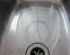 |
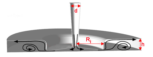 |
| A hydraulic jump in a kitchen sink. Scientists say it is a good model for an astronomical White Hole. | A schematic of a hydraulic jump. The nozzle diameter is "d", and the height of the water is "h". It is really hard to measure "h" so leave that alone for a while. |
For a flow of water as in the diagram above, the radius of the hydraulic jump Rj is related to a number of factors and exploring these would make a great EEI. But you should note that the concepts are quite difficult and the maths could be a bit daunting. The most obvious are: the volume flow rate of the jet of water (mL/s), the impact speed (which can be determined from the height of the nozzle above the plate), and the density and viscosity of the liquids. You could try using a burette, and making a series of nozzles for it of different diameters (I just took the nozzle off). Varying density or viscosity could be done using ethylene glycol (car radiator antifreeze) and diluting it with water. It has been found that surface tension has an effect so you could make up water solutions with different concentrations of detergents (not too much).
Measuring
the velocity of the water as it spreads across the plate is very hard but can be
done by high speed filming and observing the outward radial motion of micro-bubbles. Even though the theory is difficult, you may be able to determine
some simple relationships between the variables by use of graphs. I had lots of
trouble measuring the flow rate of water out of the burette (needed 3 hands) but
I think if you videoed a stopwatch and the burette as it empties you could get
accurate measurements.
 |
 |
 |
| Here's the setup. The hand belongs to Mia. Food dye was used to make it easier to see and we used a tray to catch the overflow for later reuse. | At a drop height of 10 cm the radius of the jump was 12 mm. The white tile had a side of 150 mm. You have to make the flow rate is the same each time. | But at a drop height of 20 cm (and the same flow rate) the radius was now 19 mm. If you take a photo and know the size of the tile you can work out the radius later. |
 |
 |
 |
| The effect of flow rate: when the burette read 5 mL (almost full) the flow rate was 5.8 mL/s and the radius was 15 mm. | When the burette read 15mL the rate had slowed and the radius was 10.5 mm | ...and when the burette read 30mL the rate had slowed to just 2.6 mL/s and the radius was 5.5 mm. |
 |
|
Nayana (pictured) and Amanda found that photographing hydraulic jumps was the way to go. Moreton Bay College - Year 12 Physics - May 2016. |
This You Tube clip shows the diameter of the hydraulic jump decreasing as the liquid falls from the burette (at an ever-decreasing speed). |
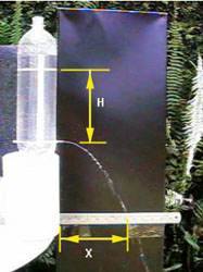
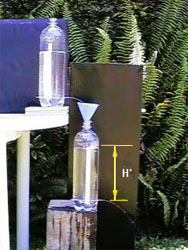
You've probably seen a demonstration of water coming out of holes in the side of a water bottle and a discussion about height and range of the water. The water speed v at the hole depends on the height H of the free liquid surface above the pin-hole, according to Torricelli's law v2 = 2gH where g represents the acceleration due to the force of the Earth's gravity. This result was obtained by Galileo's assistant E Torricelli in 1636. It is normally obtained nowadays through Bernoulli's theorem p + ½ρv2 + ρgy = C introduced by Daniel Bernoulli in his book on hydrodynamics of 1738, which appeared a century ago (C = a constant, y = height). The variables are obvious but the level of the ruler below the bottle must be controlled (there's a hint for another independent variable). If you are really keen you could do the two bottle experiment as shown below. There is a good paper on this experiment by de Oliveria et al from Brazil in Physics Education V35(2) March 2000, 110-120 (click to download).
 |
 |
 |
| Single bottle | Two bottle experiment | In the lab at Moreton Bay College. |
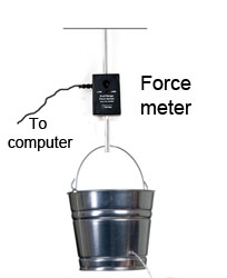
Water discharge from a leaky bucket
Whether its at hole in a dam wall or a leaky urn in
the tuckshop - leaks are annoying. But the rate of flow of water from a
reservoir is obviously dependent on the height of water above the hole (the
'head') and the size of the opening. Engineers model fluid flow through an
orifice so they can design the optimum combination when the flow is desirable,
and the design safety devices for coping with accidents when the flow is not
wanted. A great EEI can be done on this topic. I just saw a great one by
Year 12 student Steven Ettema from Brisbane Bayside State College using a bucket
of water, a Pasco force meter and a computer to collect the data. His teacher Mr
Ben Robson was very impressed.
Steven's dependent variable was the change in weight (Fw) of the water with time, and his manipulated (independent) variable was the size of the hole in the bucket (see diagram below). His development and justification of the hypothesis was breathtaking. To tantalise you I can report that is took 14.3 seconds to drain 3 L of water through a 2 mm orifice, and 2.8 s for a 6.5 mm hole. But it is not the total time that is important - it is the rate of emptying, and the shape of the rate/time graph, and the analysis and discussion afterwards.
 |
 |
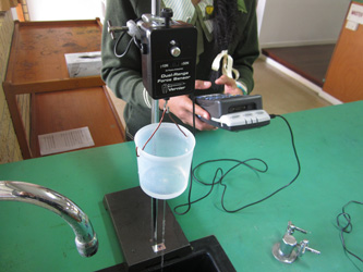 |
Setup at Our Lady's College, Annerley. |
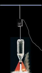
Water discharge from a water rocket
Steven's idea mentioned above can also be used
to measure the change in flow rate with time from a water rocket (plastic water
bottle partly filled with water and pressurised). When the stopper is removed
the water jets out under gas pressure. However, as the air in the headspace
expands, the pressure decreases and you would think the rate of flow gets less.
All you need to do is prepare a pressurised water rocket in a water bottle,
suspend the water rocket from the ceiling using a force meter to measure the
weight, and the remove the stopper from the mouth. As the water comes out the
force meter will give you a reading of the weight (gets less - but maybe not
regularly). You could then consider changing the starting pressure or the volume
of water or whatever you like. My thanks to Steven Ettema at Brisbane Bayside
State College and his teacher Ben Robson for suggesting this.
Water flow I - Poiseuille's Law
The study of the flow of real fluids through tubes is of considerable
interest in physics and chemistry as well as in biomedical science (flow of
blood in arteries) and in engineering. Engineers have to keep water moving in
pipes to supply cities with drinking water, and to take waste water away. They
know that the speed of the water depends on the viscosity, the diameter of the
pipe, the length of the pipe and the pressure difference. Poiseuille's Law
quantifies these quantities in the formula:
Q =
πR4ΔP / 8ηL.
You can look this up to find out what the symbols mean.
A first year university experiment is shown in the diagram below but you could do it with a Buchner flask in place of RF (below) and a plastic water bottle, stoppers and glass tubing. You hook up a vacuum pump to reduce the pressure in flask RF and when the valve "A" is opened water flows from jar CF through the pipe "T" into the flask RF. By measuring the volume of water collected in a given time for a controlled pressure and tube diameter and thickness you can look at relationships. Then vary the length of the pipe, or its thickness, or the pressure, or the viscosity and so on. What a fabulous experiment for an EEI. A paper about this experiment is available from the European Journal of Physics V27 (2006) 1083-1089. Click to download. If you do it as an EEI please send me a photo for this webpage.

Water flow II - Poiseuille's Law
Another neat way of exploring
the factors affecting flow rate in liquids is shown in the diagram below. It
could be used in university physics. The motion sensor measures the changing
height of the water column by using an ultrasound beam. These are commonly
available in high school laboratories these days (Vernier, DataLogger Pro etc).
Again, by changing the thickness of the tube, or length, or viscosity you can
measure the rate of change of height (the height of water is related to pressure
(P = F/A = mg/A = ρgh).
For high school, you could also keep pressure constant by having a small hose
from the lab tap going into the top of the column (and doing away with the
motion sensor). You could do it with a plastic water bottle, a stopper or two
and some glass tubing. What a great EEI! A paper about this experiment is available
from the European Journal of Physics V29 (2008) 489-495. Click to download.
If you do it as an student experiment be sure to send me a photo for this page.
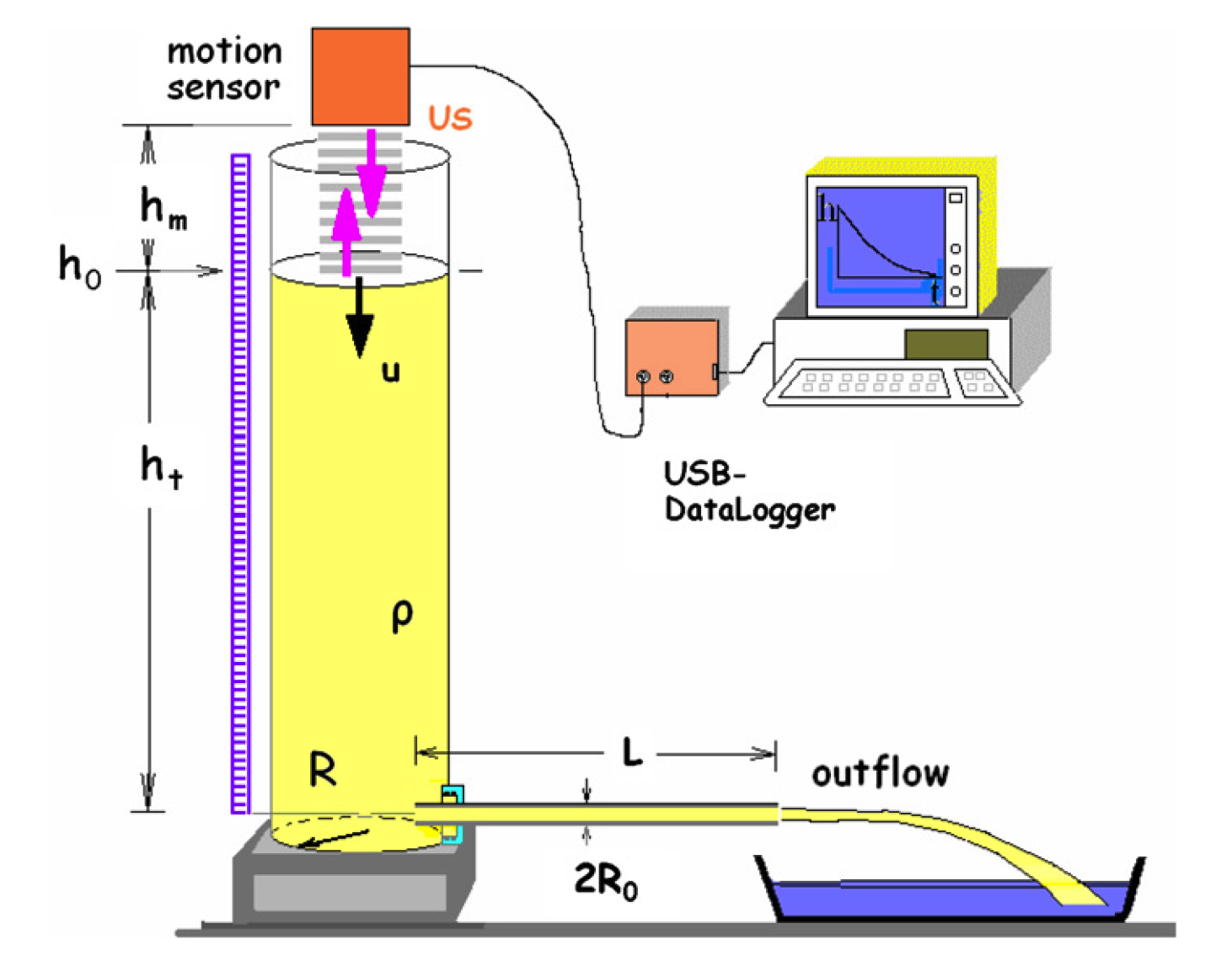 |
| The experimental setup used for the measurements, where US are the ultrasonic waves, hm, h0 and ht are the measured, the initial and the present height respectively, u is the velocity of the free fluid surface, ρ is the fluid density, R and R0 are the radius of the )container and of each pipe, respectively and L is their length (Sianoudis & Drakaki, 2008). |
Student Extended Experiment
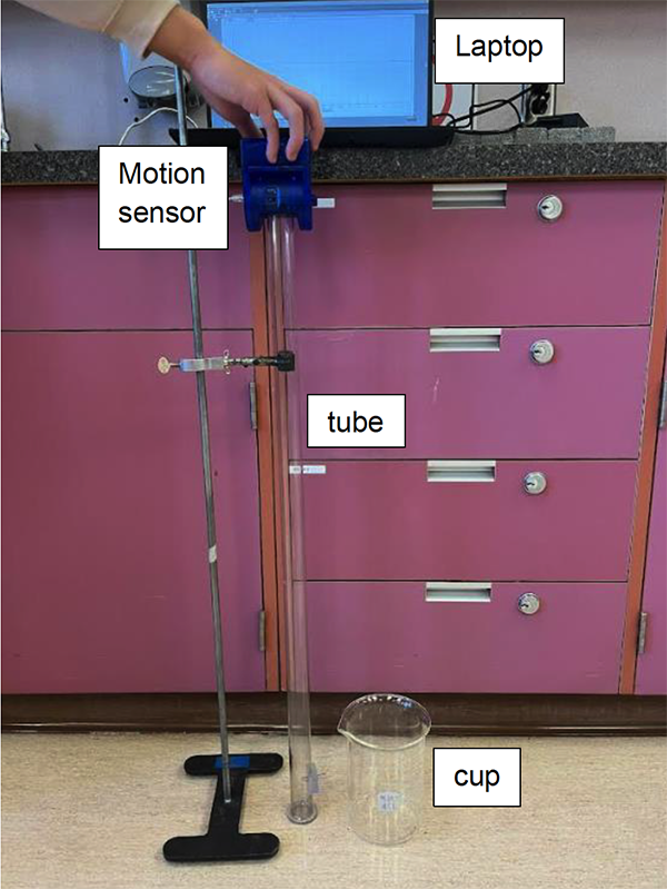
Here are some results from Tian Xie from Semiahmoo Secondary School, South Surrey, British Columbia, Canada as part of an International Baccalaureate Extended Experiment (EE). His experimental setup is shown in the photo below and is based on the image above.
 |
| Setup for the IB EE. (Tian Xie, 2022) |
His results:
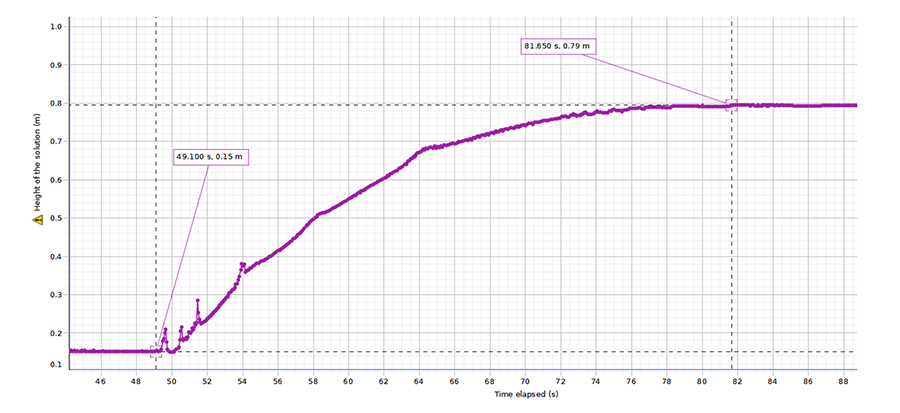 |
| An example taken from the 50% sucrose solution trial. The time elapsed is determined from the first and last flat portions of the graph. (Tian Xie, 2022) |
The following graph by Tian Xie is a part of the error analysis in which his experimental results are compared to the experimental value.
 |
| Average flowrate vs viscosity with experimental and theoretical values. (Tian Xie, 2022) |
My thanks to Tian Xie for providing his report. He has graciously agreed to making it available to read. Go to: Tianhong_Xie_IB_EE.pdf
Water flow III - Saxon Bowls
The earliest means of measuring time was by the observation of celestial
bodies (Sun, Moon, stars). However, not far behind were water clocks. One of the
oldest was found in the tomb of the Egyptian pharaoh Amenhotep I, buried around
1500 BCE. Later named clepsydras ("water thieves") by the Greeks, who began
using them about 325 BCE, these were stone vessels with sloping sides that
allowed water to drip at a nearly constant rate from a small hole near the
bottom. In a variation, the Saxons (ancestors of modern-day English, Germans and
Dutch) would place a small bowl with a hole in its bottom in a larger container
of water. It would slowly sink as water rushed in through the hole and
and finally submerge when full. The Saxons used the time it took the bowl to
submerge to limit orations (speeches).
There is a story that other service providers used such bowls to allocate their customer's time. These were still in use in North Africa in the 20th century. It is highly likely that there is a relationship between the diameter of the hole and the time until submergence (and it won't be linear so plenty of data points). However, as water enters the hole and the bowl fills you would think it would get harder and harder for more water to enter. Maybe, maybe not. Also, it would seem that as the cup sunk the hole would be further from the surface and thus experience greater pressure. I've seen these cups made from the plastic (PVC) caps they use for plumbing (see below). Buy a lot, drill holes of varying diameter and Bob's your uncle. May need one drop of detergent (why?). You could even use an old jam tin or something like that (which may give a longer sink time). Lots of errors to talk about.
 |
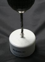 |
 |
| 40 mm PVC cap from Bunnings $1.98 each | Drill hole | Water comes in |
 |
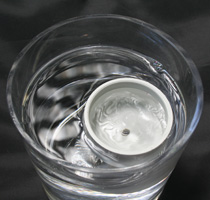 |
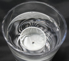 |
| Starting to sink | Almost gone | Gone |
Year 12 Physics student Codi Baker-Lahey from St Andrew's Anglican College at the Sunshine Coast, Queensland, Australia, did a Saxon's Bowl EEI in 2016. She hypothesised that as the diameter of the Saxon Bowl was increased, then the sinking time would decrease when the dimensions of the bowl and density of sinking liquid are kept the same.
She argued, in part, that a higher flow rate would result in a decrease in fluid pressure as per Bernoulli's theorem which states "if the fluid flows horizontally so that no change in gravitational potential energy occurs, then a decrease in fluid pressure is associated with an increase in fluid velocity." Of course you'd need to justify your hypothesis with more than just that - as Codi did. Her graphs are as follows:
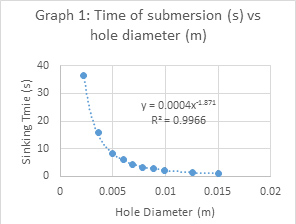 |
 |
| This graph appears to be a y ∝ 1/x2 relationship. To confirm that, Codi plotted y vs 1/x2. See the next graph. | Codi's graph is linear with a slope of 0.0002 s m2. The R2 value of 0.9969 shows it is a good fit for the data. |
Water Flow IV - The Syphon
Blood travels around your body through veins, arteries and so on. As it flows there is loss of energy due to viscous resistance with the walls of the blood vessel and this is the major source of blood pressure drop. This energy is transformed into heat. Such flow can be modelled by the use of a syphon.
With a water syphon (see below) it seems logical that the flow rate is dependent on the height of the "loop". This is borne out by experiments. However,this is not because there is a greater weight of water being pushed up the tube (because there is an equal weight of water on the other side to balance this out. It is to do with the greater length of tube and hence the greater friction involved in the flow. Poiseuielle, a French Physician, worked out experimentally the factors that determine flow rate in capillary tubes: Q = πR4ΔP / 8ηL, where L is the total length of the tube. Hence, flow rate (Q) is inversely proportional to the length of the tube. I tried three lengths of clear PVC tubing: 50, 100 and 150 cm, and kept the h3 value the same at 20 cm. This gave me h1 values of 12.5, 38 and 62.5 cm. My flow rates were 19.5, 10 and 7 mL per minute. I've plotted them below:
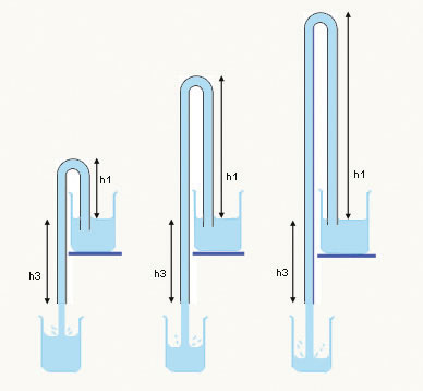 |
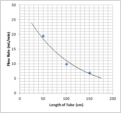 |
But this is hardly enough fro a good EEI. For a start you'd need a lot more data points (perhaps do triplicate measurements of each of five diferent heights). And you should be able to think of factors to vary besides height. "R" is the internal radius of the tube and the flow rate appears to vary with the 4th power of it. There's an idea.
Water splash heights
When you stand in the rain sometimes the raindrops feel nice other times they hurt. But what conditions determine the force of the impact. Imagine a single drop of water dropped to the ground from a few metres high. Prior to the impact, the water drop possesses only kinetic energy. After it touches the surface, the drop is deformed so that a shock wave spreads radially outward near the surface, increasing the surface area of the drop, thus increasing its surface energy. For moderate initial energies (low drop heights), the surface tension will be able to absorb the initial kinetic energy like a spring, and the restitution force will cause the drop to bounce. The scientific term for this recoil is in fact "bounce". For higher energies (higher drop heights), the surface tension is not sufficient to stop the outward motion as the drop spreads upon impact and forms small droplets that splash upwards. We know that the speed of a falling drop is related to its drop height, which determines the resultant bounce and/or splash heights.
This is of concern to environmental scientists as the erosion of soil and "crusting" is a function of their size and energy. Engineers developing automatic fire extinguishers also need to know how speed and droplet size are related because they want to get the right amount of water to the seat of a fire (but they talk about sizes like 200µm to 3000µm and speeds of up to 30 m/s - and this is clearly not suitable for a high school lab).
This suggests a great EEI though. You could investigate the bounce and splash heights of a water droplet as a function of its drop height and diameter. It seems that you do not have to worry about the droplet reaching terminal velocity before it strikes the ground as water droplets of 2mm diameter take at least 5 metres to reach terminal speed.
Firstly, how to make a good droplet. A burette works really well.
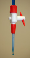 |
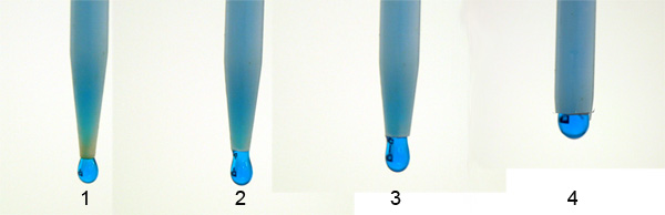 |
| Burette tap with a plastic tip. The water has been coloured with food dye. | Successive photos of a burette tip cut off in stages to form bigger drops. Photo 1 shows the original tip; 50 drops from this had a mass of 2.156 g or 0.04312 g per drop. This equates to a volume of 0.04312 mL, and if you consider it a sphere it would have a diameter of 4.35 mm. Drop 2, mass 0.05036 g (diameter = 4.58 mm). Drop 3, m = 0.05414g and diameter = 4.70 mm, and Drop 4 is 5.18 mm diameter. Courtesy of Moreton Bay College. |
How to measure drop diameter? If you ever do titrations in chemistry you'd know that 1 drop from a burette is said to be 0.05 mL. If you treat this drop as a sphere of water you can work out its diameter. I'd let 100 drops fall from a burette or dropper into a beaker on an electronic balance; then calculate the mass and hence volume of one drop. To get bigger drops just cut a little bit off the tip of the plastic nozzle (see above). These are disposable and are as cheap as chips. You can get them from LabPro if you are in Australia.
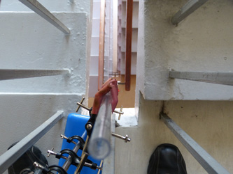 |
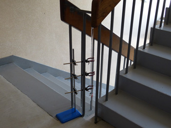 |
Here's the setup used by colleague and physics teacher Dave Muir at Portobello High School, Edinburgh, Scotland. The long drop is through the gap in the stairwell. |
To make sure the burette didn't fall Dave used three clamps. He said that somehow the English teacher on the ground floor got rather wet as he walked past. Kids will be kids. |
Measuring bounce and splash heights is another thing. Dave suggested we use a tray of water 5 cm deep and a sheet of black cardboard with a ruler attached. The splash height was obvious from the droplets on the black cardboard. To see the bounce heights he videoed the with an ordinary camera and scrolled through the frames to see the bounce height (VLC Player works okay for this). This is not necessary if you are just doing splash heights. You can see Dave's video here. This EEI would be so much fun.
 |
 |
Dave's photos taken as screen captures. Here the drop height was 90 cm and you can see the bounce height of 2.2 cm (7.2 cm ruler reading less the 5.0 cm offset for the water level). Likewise, the splash height is 10.3 cm (15.3 - 5.0 cm). |
From 1.5 m high, the bounce height is 2.7 cm (7.7-5) and the splash height is 12 cm (17-5). Dave also tried a water depth of 1 cm and got different results - so that's another variable to consider. |
Fun
with a toy helicopter
If you want to play with a remote controlled
helicopter and do a Physics EEI at the same time - here's an idea suggested by
our colleague Michael Liebl, Physics teacher at Mount Benedictine High School,
Elkhorn, Nebraska, USA. A helicopter flies by means of the thrust that is
created by the rotation of the blades of a main rotor that is mounted on a shaft
above the fuselage of the aircraft (see below). As the blades rotate, an airflow is created
over them, resulting in lift. This raises the helicopter. Newton's third
law requires that the air in turn exert an equal force upward on the rotor. For
a helicopter to hover, the force exerted by the rotor blade on the air must be
equal to the weight of the helicopter.
With a few simple assumptions and basic
laws of physics, it can be shown that the relationship between rotational
frequency of the rotor blade (f) and the mass (m) of the helicopter is: f 2 = mg/(8p3rl2 R4 ) where r is the air density, R is the rotor radius, and l is a constant. A great EEI would be to buy a remote controlled helicopter off ebay for about $19, tape it to the pan of an electronic balance and vary the
rotational speed (how to measure? You decide!). You're not trying to prove the
formula but look for relationships between various quantities such as mass,
frequency, radius, blade angle and so on. What fun! Here's an article from The Physics Teacher that gives a bit of the theory.
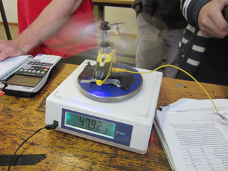 |
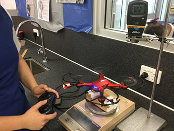 |
| The students at Villanova College, Brisbane, said the speed of the rotor in this photo was 2600 RPM. | Kerry-Lee and Madi used a quadcopter from Jaycar ($90) that worked well. The digital stroboscope ($90) measures reflected laser light from reflective strips stuck on to the blades. |
| Quadcopter in action. You can see the stroboscope reading (RPM) and the scale reading on the balance (negative grams). You could even plot these data to see the relationship (if any). My thanks to Kerry-Lee at Moreton Bay College. |
Lift of a flat surface in wind
You may have seen the roof a house lift off in a storm. Sometimes it is
the low pressure created on the top of the roof that causes it to lift off.
However, with awnings and carport roofs it could be the wind lifting from
underneath. What would be interesting to find out (and make a good EEI) is to
see how the wind speed affects the lifting force of a flat roof. Perhaps you could measure the upward (or downward) force on a
flat surface by using an electronic balance that supports a pillar with a flat
surface attached at the top, push the 'tare' button, and turn the fan on. Voila!
In terms of physics theory you would need to consider Bernoulli's Principle in your investigation. There is a heap of stuff on the internet. Just Google "Bernoulli's Principle lift of roof" and you'll see plenty of pages with examples and calculations. One that seems quite good and has a worked example is here.
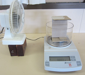 |
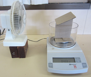 |
| Tried it out at Moreton Bay College with corrugated cardboard and seemed to work fine. Zero degrees gave 0.003 g scale reading (0.03 mN) but it fluctuated. Must try a better design. | You could vary the angle. At 30°, the scale reading was 0.408 g or 4.08 x 10⁻⁴ kg (about 4 mN). How would this change if the surface area was bigger? |
There are 3 variables to consider (one DV and three possible IVs):
1. Lift (the dependent variable DV);
2. Wind speed
3. Area of roof
4. Angle of roof
To change wind speed you could adjust the setting on a fan (off, 1, 2, 3). That would give you 4 "treatments" or data points but they are not a measured physical quantity (but just someone's idea of fast and slow). Five points would be better, so you could shift the fan away from the "roof" to make the speed lower. To measure the speed (important for an EEI) you could use an anemometer (wind speed meter) that most schools seem to have (if not in Science, try Geography). Alternatively, there is a windspeed app "Wind Meter" ($0.99) for iPhone that is amazingly accurate (I compared it with a $99 Windtronic and the results were in excellent agreement). It's also available for Android. It uses the microphone as a sensor and the loudness of the sound is a measure of the speed. If you can't get steady results from the scale it may be that the weight of the device is too light and it is jumping up and down a bit on the pan. Make it out of something a bit heavier.
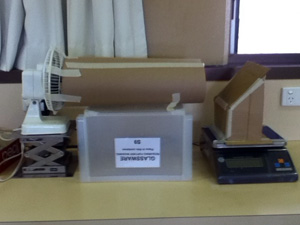 |
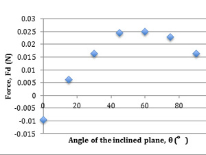 |
| Here's Allie's setup for her 2013 Year 12 EEI. | ...and one of Anwen's graphs taken from her EEI. |
What more to say: a simple but socially relevant investigation set in the context of houses having their roofs blown off. Cool!
UNIT 2.2 WAVES
Loudness and Distance
Loud music can cause hearing damage. The closer the source is to your ear the louder it sounds. That's why earbud headphones can be bad for your health. This EEI looks at the relationship between loudness and distance. In essence, you just generate a fixed sound and measure its loudness or sound pressure level (SPL) with a microphone or as you gradually move it away from the source. But be careful with the theory here. The sound intensity (I) is different to the sound intensity level (L). Intensity (I) is inversely proportional to the square of the distance between the loudspeaker and the microphone.
Sound intensity level (L) is the perceived sound intensity taking the response of the human ear into account. The response of the human ear to different intensities at fixed sound frequency is close to being logarithmic. The sound intensity level (L) is proportional to the log of the ratio of sound intensity to the threshold of hearing intensity (L = 10 log (I/Io). [For more see the article by Alan Bates of John Cabot University in The Physics Teacher, V52, May 2014, p302].
For a point source of power P emitting sound uniformly in all directions I = P/(4πd2). The "π" symbol is pi. In our case we assume the loudspeaker behaves like a point source that emits sound in the forward direction only, that is, I = P/(2πd2). The equation L = 10 log(I/Io) can be rewritten as L = 10 log(P/(2πd2)/Io) = 10 log(d-2) + 10 log((P/(2π)/Io) = -20 log(d) + 10 log(P/(2π)/Io). This takes the form of a linear relationship y = mx + c. So if you plot log d vs L the slope "m" will be -20 and the y-intercept "c" will be 10 log(P/(2π)/Io), so you can solve for power P. The value of Io is 10-12 W/m2. Let's try that.
Two things are necessary: 1. A source of sound. The simplest thing would to be use Audacity on your computer to generate a set frequency (say 3000Hz) played through some earbud headphones (well, just one earbud; hide the other one under a pillow). Make sure you keep the sound at the same level between tests. 2. The other thing is a sensor to measure sound pressure. Audacity can measure loudness but it doesn't calculate SPL values; it just converts the analogue input to a digital signal and assigns 0dB on the recording level meters to a certain input level, which corresponds to the maximum value of the digital signal. So forget about that. You can get a great SPL meter app for the iPad and iPhone for a cheap price. Two researchers - Chucri Kardous and Peter Shaw - from the National Institute for Occupational Safety and Health - tested 100s of apps for performance and accuracy. Their results were reported in the Journal of the Acoustical Society of America V135, EL186 (2014): "Evaluation of smartphone sound measurement applications".
The highest rated app was the SPLnFFT for $4.99. This was the only app to absolutely nail the results each and every time. It passed all four tests with flying colors. In fact, this app's results were so close to the results obtained using the $2,000 noise meter that the tiny differences between the two were probably due to sampling error. Other excellent ones were SoundMeter $24.99, Noise Hunter (iOS4) $7.49, NoiSee (iOS5) $1.29. They said the microphones on the Android and Windows devices were not very good (but that may have changed by now). I used NoiSee which was terrific (see photo below), but Noise Hunter was much much better as you could save and email the the readings and it gave you peaks, averages and standard deviations. My recommendation. My thanks also to Sophie, Claire and Renee from Moreton Bay College for testing this out in their terrific EEI.
 |
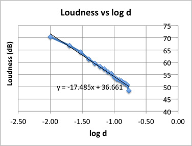 |
| The earbud speaker is 1 cm from the iPad's microphone. The app being used is NoiSee as it was the cheapest of the recommended ones ($1.29). If I wasn't on a teacher's wage I would have bought the SPLnFFT for $4.99). It is very easy to use - so they say. I measured the loudness every 1 cm up to 10 cm. Update: I eventually bought one and it works well. | Here's a graph of my results. I was hoping for a slope of -20 but ended up with -17.5. The main point is that it is failrly linear for a plot of L vs log(d) which means that the loudness varies with the log of the distance. It cuts the y-axis at 36.7 dB and this is a measure of the power of the source. |
A good frequency to try is 3 kHz. This value is used because the human ear is most sensitive to frequencies in the 3.0 to 3.5 kHz range: the ear canal, treated as a closed column with length 2.5 cm, has a resonance frequency equal to 3.3 kHz. But don't quote me - get a proper reference. The distance between the loudspeaker and the sound level sensor could be varied (say) from 1 cm to 50 cm. It sounds close but the background noise wouldn't intrude. MBC students tested it out to 6 metres but got all sorts of background noise interferring. I also investigated different frequencies (see below).
Sound intensity and distance - frequency effects examined
It seems obvious that the further you are away from a loudspeaker the less
loud it will sound (see above). You textbook will tell you that the intensity level
of a sound is directly proportional to the logarithm of the inverse square
of distance from the sound source. But is this true for all frequencies or is
this just a general relationship. You can hear the thumping bass from an
outdoor rock concert miles away but the higher frequencies seem to diminish
quickly (however, there are too many variables to make that an EEI). How does
the relationship stand up over say 10 cm or 10 metres? You have to be cautious when using big distances as external sounds intrude. Here are some student results.
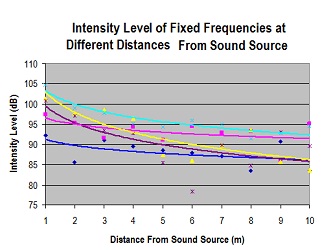 |
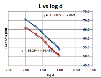 |
| Some student results. Each colour represents a diffferent frequency. You can see that the greatest change is over the first meter. You'd then need to plot log d vs Intensity level (dB). | Here's a plot of L vs log d (as above) but at two different frequencies (blue 3000Hz and red 1000Hz). The slopes are the same but perhaps the sound meter (NoiSee) is more responsive to the 3000Hz - which is the most sensitive for humans. Thank you Sophie, Claire and Renee. |
Singing wine glass
You can make a wine glass sing a pure tone by rubbing
your degreased and wetted finger around the rim. Vibrations are set up in the
wall of the glass and resonance occurs in the air column. When you increase the
volume of water inside the glass the frequency of the sound changes
(increases/decreases? - you find out). A lot of it is counter-intuitive! But is the pitch proportional to the circumference, the
diameter of the glass or the amount of liquid in the glass? Physics books give wayward opinions and you could finally work out
who is right and what factors are involved. Capture the sound on a CRO and
work out the frequency. Four variations you could try are shown below. The last
one has a solid column in the glass so there is less water but the same water
level. Or you could compare liquids of different density or viscosity; or
non-polar (hexane) with polar (ethanol). Don't try to do too many variables or
you'll run out of time.
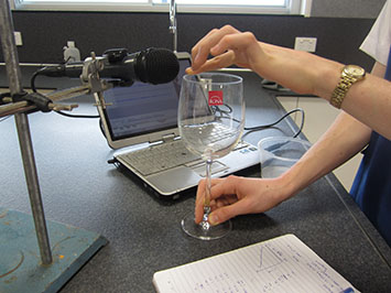 |
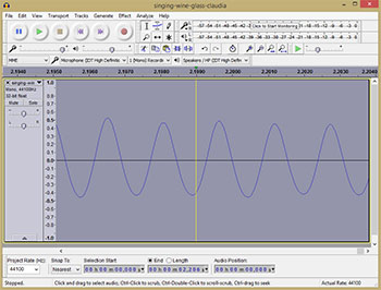 |
| Setup for generating and recording sound waves. My thanks to Alexa from Moreton Bay College. She had some ethanol in the plastic container beside the computer. This helps removing any oil from the fingers. | The sound wave captured on Audacity. With our empty wine glass the predominant frequency was 720 Hz. A sample of the sound can be downloaded here if you want to experiment. Wave made by Claudia at MBC. |
Here's a stimulus for developing a great EEI based on the Singing Wine Glass. My
thanks to Physics teacher Steven Anastasi from The
Cathedral College, Rockhampton, Queensland: "One would expect that a
singing wine glass behaves like a closed pipe, but a few simple tests challenge
this fact. For one thing, filling the glass with water would imply that the note
goes up, not down. Does it? That said, the length of a wine glass is very short,
so the frequency might be so high you just don't hear that note. Perhaps these
days there is software available that can 'hear' well above the range of human
hearing, and this would be worth investigating by doing a theoretical analysis
of the frequencies expected, then searching for them with technology."
Yet there
remains the question of what variables influence the frequency of the singing
wine glass, and testing the frequency heard is just one aspect, and a little bit
simple for a thorough going physicist. Is it the thickness of the glass? The
volume of water, the height of water? The percentage of water from the
top/bottom of the glass? Is it a coupling of the water to the glass? Is there a
temperature effect? Is it
predictable. Indeed, the holy grail of singing wine glasses is to arrive at a
formula that predicts the frequency that might be heard, for well justified
reasons. Your object ought to be to arrive at an answer. This might be
discoverable using your fancy calculator, but that is maths (barely) not
physics. In the end you should be able to provide reasons for its behaviour,
based on your personal observations, and verifiable by prediction based on
equations or by trend." If you think that the pitch is lowered when you add
water to the glass you are right (diagram 1 below); but if you say this is because the added
liquid is forced to participate in the vibration of the glass wall, then
wouldn't you get a similar result for diagram 2 below? Well you don't - and
therein lies the beauty of this for an EEI. There is a good little article in the Physics Teacher December 1990.
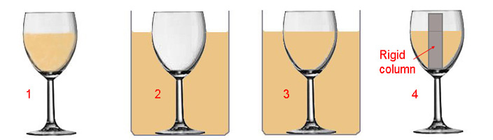 |
| Some possible variables. |
The reverberation time of a large hall
You are probably familiar with the way some rooms echo whereas others always
sound really quiet. The best measure of this acoustic property of a room is
known as reverberation time. Reverberation is the persistence of sound in a
particular space after the original sound is stopped. A reverberation, or
reverb, is created when a sound is produced in an enclosed space causing a large
number of echoes to build up and then slowly decay as the sound is absorbed by
the walls and air. The reverberation time (RT60) is the time
required for reflections of a direct sound to decay by 60 dB below the level of
the direct sound. The reverberation time receives special consideration in the
architectural design of large chambers, which need to have specific
reverberation times to achieve optimum performance for their intended activity.
This makes a great EEI.
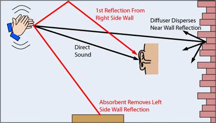

Not only can you measure the reverberation time of a number of different rooms (laboratory, classroom, large lecture hall, auditorium, sports hall) but you can make measurements from different parts of the room. Best of all, you can calculate the theoretical value for RT60 using the formula RT60 = 0.161V/ S(a×s) where V is the volume of the room in m3, a is the area of each absorbing material in m2, and s is the absorption coefficient for each material. All you need is a stopwatch, a ruler, a sound pressure sensor (connected to a computer is good) and something to make a loud noise. Toni Tran from Victoria Point SHS popped balloons with a pin for her sound source and her RT60 values were: hall 1.5 s, classroom 1.0 s, sports hall 1.8 s and so on.
A more sophisticated setup for measuring sound pressure level (loudness) is using the Audacity program on a computer. In this case you would start recording and then pop a balloon. You will see a spike on the waveform which levels off to zero as the sound dies away. Trim the waveform by deleting the quiet parts either side. Then go to "Effects" menu and select "Normalise". Check the DC Offset box to remove offset, and enter -1.0 as the maximum amplitude. That will reduce the peak amplitude to a managable level. In the "Audio Track" menu to the left of the wave, you can select "Waveform (dB)" so that the scale is now in dB instead of from 0 to -1. Audacity sets the peak to 0dB and the middle horizontal axis to -60dB which is designed for working out reverberation time (see below). Just note the time elapsed from the big peak to where the line crosses the -60dB central line. Use a ruler as the graph should be a straight line. I added the yellow line to make the slope clear.
 |
| The balloon pop began at 0.05 seconds (0 dB) and reached the -60dB level at 0.45 s. So the reverb time is 0.40 s which is fairly typical for a lounge room at home (where I took this sample). Short reverb times like this are excellent for speech and music at home (but hopeless in a concert hall). I measured the reverb time for a new and old lab at a school I visited. The old lab was 0.9 seconds (good) but the new one was 1.7 s (awful - too much echo and was much noisier than the old lab). The recommended RT-60 cut-off for classrooms is 1.0s so it indicated that sound-absorbing panels were needed. |
Guitar Strings and Mersenne's Law
You should be well aware that as you tighten a
guitar string it's pitch (sound frequency) increases; and the thick strings
wound with copper produce a lower frequency than the lighweight steel or nylon
ones. This is the basis of Mersenne's Law: the fundamental frequency of a
vibrating string is proportional to the square root of the tension and inversely
proportional both to the length and the square root of the mass per unit length.
You could investigate this for yourself but the Law is only the starting point;
it's no good just proving the law by using a recipe-style experiment - that's
hardly the recipe for a good EEI.
For some practical suggestions for this investigation go further down this EEI webpage until you hit "Guitar Pickups" where I talk about making a sonometer. I made one from a piece of pine about 120 cm long. As far as the string goes I suggest going to a guitar shop and get a G-string as it is the thickest (0.016 inch - commonly said to be "16 thou" referring to it's diameter of 16 thousandths of an inch). For the weights hanging over the end I used some from a weightlifting kit. You could start with the slotted brass masses from school (up to say 500 g) but after that you really need big steel masses. These are cheap from shops like A-Mart Sports if you haven't got any others. I'd increase the mass in 0.5 kg increments up to say 3 kg. That will give you a tension of 4.9 N to 49 N. You need a microphone and plug it into the computer sound port and use the program Audacity (free to download) to record and analyse the sound.
Some more suggested research questions have been made by Physics teacher Stephen Pinel to whom I am most grateful:
- As a string is tightened, does the spread and amplitude of harmonics change?
- If the string length changes (same tension) does the spread and amplitude of harmonics change?
- As a string cools/heats, does the spread & amplitude of harmonics change?
- If two strings create a particular interval (like C-G), do they stay in tune if their temperature changes?
 |
 |
 |
Comparison of Musical Instruments - effect of temperature
Here's a stimulus for developing a great EEI in the
context of The Physics of Music. My
thanks to Physics teacher Steven Anastasi from The
Cathedral College, Rockhampton, Queensland: "Musicians usually tune their instruments at the
last moment. Might there be a good reason for this? Compare and contrast the
physics of a woodwind instrument (e.g. recorder) to that of a stringed
instrument (e.g. guitar). What differences in pitch might you expect of each
instrument in changed temperature conditions? This might be considered from
several perspectives - the air temperature, or the temperature of the
instrument, preferably both.
You know from theory that the frequency of the
woodwind instrument is related to the speed of sound, and from thermodynamics
that the speed of sound in air is different when it is colder. How would this
affect the note, and can you describe this with equations? Similarly, does a
guitar string 'speed up' or 'slow down' when it is cold? Does the frequency also
depend on the speed of sound in air? Would a woodwind player and a guitarist
have the same tuning issues if they gave a concert in a freezer? How could a
woodwind player tune his/her instrument? Your task is to consider this from a
theoretical perspective, then test it in an experimental setting. Variables that
might be considered include whether end correction of the woodwind instrument
changes against the controlled variable. Does it matter which note you are
testing? Is there a connection between end correction and the note? Could you
'correct' the instrument by adding or removing the tip of the wind instrument?
Smoke Rings - the physics of the vortex
I bought a Zero Toys "Vapor-Ring" gun on-line for $23. It produces vapour
"smoke" rings about 5 -10 cm in diameter that shoot out a few metres. They are
not really smoke but are condensed water vapour clouds produced by a mist of
cold alcohol vapour in the gun. It even has a blue LED light and ray-gun sound
effect. This suggests a possible EEI.
I don't think you'd have much of an EEI if you just had fun with them and
tried to make the biggest or fastest ring you could. You need a hypothesis about
some variables that you can justify with reference to physics principles, and a
means of manipulating these variables.
Instead of buying the Zero Toys Vapour
Ring you would be better making your own so that the variables can be
manipulated more easily. There are plenty of instructions online to choose from;
but a can (eg soup, canned fruit) with a balloon over the open end and a
circular vent in the other is a good start. When you gently flick the balloon
end of your vortex launcher, a transparent ring of spinning air will shoot out
of the hole (you can feel it and blow out a candle metres away). You need to
make the ring visible so a smoking incense stick may help (or make clouds from
dry ice in water and inject into the can through a tube). How does the hole size
affect the ring? How does greater stretching of the balloon affect the ring?
Good EEI variables.
 |
 |
| A MegaBlaster smoke ring gun from Zero Toys. Wow! | Backyard smoke ring using a rubbish bin. |
For more control of your variables replace the rubber drumhead with a large
bass loudspeaker hooked up to a power amp driven by your computer's audio
output. This isn't really necessary to have a good EEI but if you are really
keen - it could be good. Using a waveform generator like Audacity you
could control of the impulse waveform applied to the vortex generator. The
waveform is a single pulse. The steep leading edge of the pulse creates the
vortex. You may want to try pulses of different shapes. The loudspeaker cone
should move forward quickly, then suddenly stop, then slowly return to its
original position (like wave 2 below). Here are some waveforms to think about.
 |
| 1 is a square wave; 2, 5, 6 & 8
are sawtooth. Waves 4 & 7 are triangular. Wave 3 is not so sudden as wave 2. Waves 4 & 5 are more gentle. |
A square wave (1) will give a fast rise and should give a high velocity. The
repetition rate of the square wave generator will allow you to create a train of
vortices. But you could try creating various shapes with a waveform editor as
shown above. Using Audacity you can select Generate/Tone from the main
menu and choose from a small range of shapes (sine, square, sawtooth) and maybe
set the frequency at 0.5Hz for a start. If you want to really get into the
effect of the waveform on the vortex you will need an "arbitrary waveform
editor" (AWE) where you can change the shape to your heart's desire. A fabulous
one is the "Bitscope Digital Storage Oscilloscope" package which has an AWE
built in. Just choose the "Ramp" wave-function, set the frequency to 1.00 Hz and
adjust the "symmetry" from 0% to 100% and the waveforms will change as shown
below. Bitscope www.bitscope.com is an
Australian company from St Leonards, New South Wales.
 |
 |
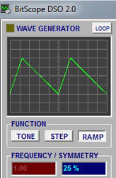 |
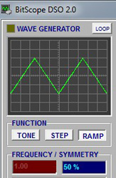 |
| Some screen captures from a Bitscope. The symmetry has been changed from 0% (sawtooth), to 10% which gives a less sharp rise, to 25% and 50% which are less sharp again. I used the BitScope from Moreton Bay College, Brisbane. | |||
Lastly, the physics of it all. The Physics Teacher journal (V49, Nov
2011, p489) suggests the equation relating vortex velocity and diameter is v =
k/2πd,
where k
is a constant of proportionality, and d is the diameter. You'd probably have to
video the train of rings to work out their velocity.
Tuning Fork Rotation and Jet Engines
If you strike a tuning fork and rotate it as you hold it up to your ear, you will hear the sound alternating between loud and soft. You should find four positions where the sound is loud, alternating with four positions where the sound is soft (about 5 dB lower). See the diagram below.
This can be explained in terms of interference effects. Each tine of the fork produces a pressure wave which travels outward (at the speed of sound). The compressions have a pressure higher than atmospheric pressure, while the rarefactions have a lower pressure. At some angles the high pressure areas of the two waves coincide and you hear a louder sound (constructive interference). At other angles, the high pressure part of one wave coincides with the low pressure part of the other (destructive interference). That sounds logical and simple enough.
 |
 |
 |
The various sound levels around a tuning fork are due mostly to constructive and destructive interference. |
This position of the tuning fork should give a loud sound. If the tuning fork is rotated through 90° it should also sound loud. |
At about 45° it seems to go quiet but I get the quietest at 54°. Don't believe me? Well try it for yourself. |
However, if you sound the tuning fork at arm's length from your ear and rotate it about its long axis you will only hear two maxima and two minima (not four). These two situations are known as near-field (close to your ear) and far-field (arm's length) sounds.
Naive attempts at explaining the radiated sound field in terms of compressions, rarefactions, and interference effects are unable to explain the results very well. Many physics texts attempt to explain the sound field close to the fork do so in terms of constructive and destructive interference effects but the tines of a tuning fork are almost always separated by a distance much smaller than half a wavelength of the sound emitted, which means that interference effects should be noticed only at significant distances from the tuning fork. Furthermore, the minima are not symmetrically spaced at 45° from the plane of the fork instead the first minima occurs at approximately 54°.
If you connect up a microphone these patterns may be examined on an oscilloscope. This suggests a great EEI. Rather than using a microphone, a loudspeaker can be used as it better captures the pressure waves. You need to work out a way to hold the tuning fork in position at a certain distance from the speaker, be able to rotate it in measured increments, and be able to strike so that it vibrates the same each time. I'd try clamping the tuning fork to the bench and moving the loudspeaker around. This will be no easy task. The best place to strike a tuning fork is about 1/3 of its length from the tip. You get a fairly clean fundamental. Look up how to hit it. To see how a fork vibrates you really need to look at a video at:
http://www.youtube.com/watchv=m7xUtR2qevA.
You shouldn't expect to come up with an exact model for how the pressure waves interact, but you should be able to manipulate and observe variables, analyse the data and evaluate the findings in terms of physics theory. Don't expect to do what many physicists can't. Lastly, you may wonder what practical use is all of this. One example: the turbulent flow of jet exhaust gases from a rocket engine can be modelled as a quadrupole source based on an understanding of gas pressures around a vibrating tuning fork.
Refractive Index and Temperature
Since the density of a liquid usually decreases with temperature, it is not
surprising that the speed of light in a liquid will normally increase as the
temperature increases. Thus, the index of refraction normally decreases as the
temperature increases for a liquid. For many organic liquids the index of
refraction decreases by approximately 0.0005 for every 1°C increase in
temperature. However for water the variation is only about -0.0001/°C. A good
EEI would be to examine the relationship between RI and temperature for water
and perhaps other liquids. Does it vary regularly with temperature; is it
related to the coefficient of volume expansion; do solutions of ionic or
molecular solutes have any effect and, if so, why? The possibilities are
endless. You need to get hold of a triangular tank which can be filled with the
liquid and a laser beam shone through it. Lie it flat on a hotplate and away you
go. You could easily make one from microscope slides and epoxy glue or silicone.
Before you get too far consider whether you can measure such small variations in refraction. Also, give some thought to which of the two set-ups below would be easier to analyse. Just a reminder about safety with laser pointers with an output greater than 1 milliwatt. An amendment to the Queensland Weapons Act 1990 (known as the Weapons Amendment Act 2011) restricts the possession and use of a laser pointer with an output greater than 1 milliwatt to persons with a genuine reasonable excuse. A reasonable excuse is defined in the Act and allows members of recognised astronomical organisations and people who have genuine occupational reasons to have possession of a laser pointer with a power output of less than 20 milliwatts. School laser pointers should be okay but you would need to check if you are planning to using one from home. See Weapons Amendment Act 2011.
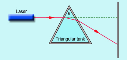 |
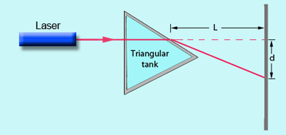 |
|---|
Refractive Index of a liquid:
another method
Another method of measuring the refractive index of a liquid is shown below.
A laser beam is shone on to a piece of flat glass (eg microscope slide) placed
horizontally in a dish. The beam reflects on to a wall and all necessary
distance measurements are taken. While the laser is held rigidly in the same
position, water (or any liquid under test) is added to the dish to a measured
height above the surface of the glass and two reflections are seen on the wall:
one from the surface of the water and one from the interface between the water
and the glass slide. Again all necessary measurements are taken. Using some
fairly straightforward geometry the refractive index of the water can be
calculated.
How to make this an EEI? You could consider making a series of
measurements at different water depths and plotting them to see if RI is
constant over the range of depths. The accuracy of the smaller depths can be
commented upon. You could always perform this on a hotplate as in the above
experiment and look at RI vs temperature, or you could think of something more imaginative. My thanks to
Prof. Shyam
Singh, Department of Physics, University of Namibia, Windhoek, Namibia for this
suggestion (Physics Education, March 2002, p152). Read about safety in
suggestion above.
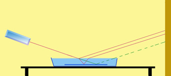 |
|
Firstly, without water.
Clamp the laser in a stand and make sure the glass is dead level. |
Then add some water and
you should get two reflections. The green dotted line is the original. |
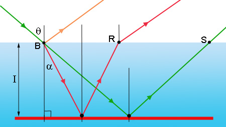 |
Simple geometry should
allow you to calculate RI. The three rays will strike the wall some
distance away. Note this distance and the height of the laser spots. |
Refractive Index and
Concentration
A mirage is where you see an object that is on the ground in the
distance but it looks like it is either floating above the ground or reflected
off the surface. It is a result of the different densities of air above the
surface caused by heating (as above). However a similar effect can be seen when
you shine a laser into a tank containing concentrated sugar solution on to which
a layer of water has been gently poured; the light bends down towards the more
concentrated region. A good EEI would be similar to the one above but to vary
the concentration of solute rather than temperature. Some experiments seems to
show a linear relationship for sugar and others a curve (who to believe?).
Others show a linear relationship for a while and then a curve.
An
interesting paper by physicists Yunis and Rahman from the University of
Agriculture, Malaysia published in Applied Optics (V27 (16), 1988 has some good
practical ideas (click here to download). I also read on one site "I think
it's worth bearing in mind that the refractive index is mostly a matter of
dielectric constant so it typically has a lot to do with the electric charges in
the material". That suggests a comparison of ionic (sodium chloride) vs
molecular (sugar) solutes; or even monoprotic (Na+) vs diprotic (Mg2+)
ionic solutes. Read about laser safety in the EEI above.
 |
 |
| See how the laser beam bends down as it travels through a sugar solution with a high density at the bottom. | One student's results show a non-linear relationship for sugar but this is not what everyone gets. |
Double reflections in a glass window
You may have noticed that when you look at yourself in a glass window
pane at night (from the inside) you see your own image plus a fainter one around the edge of it (see the image of the cat below). This is a double reflection. It can be explained by the diagram below (right) showing how the incident ray of light reflects back off the outside surface, but the transmitted ray passes into the glass and reflects off the bottom surface of the glass. If we say the incident ray has an intensity of 1.00 as in the diagram, then the reflected ray is about 0.045 (ie about 4.5% of the incident intensity). The second ray that reflects off the back surface has about 4.5% of the intensity of the transmitted ray (0.045 x 0.995 = 0.043). Together, the two rays add up to about 0.088 (8.8%). This is not a lot and your eyes are tricked into thinking it is a lot more.
 |
 |
|---|---|
You can see two reflections of "Buster" in the window. |
For an angle of incidence of 30°, 4.5% of light is reflected off glass. |
Water is not as reflective. The reflection in water at an incident angle of 30° is about a 2.2% (there is no back reflection, unlike glass). If you look into a pool of water you can easily see the reflection of the sky during the day; but at night you probably won't see any stars (but you may be able to see the reflection of the moon). Why no stars? A 2.5% reflection in water (= 1/40) reduces a 1st magnitude star's brightness to about 5th magnitude - and these are very hard to see in the night sky anyway.
A great EEI would be to see how the reflection varies with angle of incidence. We know that for an incident angle of 0°, the intensity is given by [(n-1)/(n+1)]2. For glass (n = 1.52, this equals 0.043). Your project would be to see how the intensity varies by incident angle, for water and glass. What sort of light do you use? What sensor do you use to measure the intensity? How do you stop water rippling? Should the water be in a glass container? Should the glass lie on something black. What happens if you put grease on the back of the glass to stop back reflections?
Refractive index of ice
Just as glass and liquid water cause light to refract, ice will do this too. This could make a fascinating EEI if you want something a bit different.
Refraction by ice is of huge importance to astronomers and environmental scientists. Water is a dominant building material for solid celestial bodies: it makes up the polar ice caps on Mars and is a major component of interstellar 'dust'. Astronomers use radiation in the Far Infra-red (Far IR) to penetrate this dust but they need to know a lot about how light refracts as it passes through. Here on Earth the optical properties of clouds are also critical: we know that Cirrus clouds are composed of water and ice and that they play and important part in regulating the Earth's climate variability. And what simpler way is there of measuring the thickness of Artic ice (even 2 km thick) than by sending radiation into the ice and measuring aspects of its refraction and reflection.
Refraction in ice depends on the wavelength of light being used. This is common to most media. For instance the RI (at -7°C) is 1.313 for violet light (400nm) falling to 1.308 for red light (650nm) and 1.280 in the Near IR (2000nm) but then goes up. This is not a suitable variable for a high school lab. As far as varying temperature goes, the RI also goes up and down. But it is all so complex and many PhD projects have been done trying to come to terms with it.
For an EEI you could compare a couple of ways of measuring RI in the high school lab. The simplets way is to make a small slab of ice (a rectangular based prism) and shine a laser through it, noting the angles ofincidence and refraction (see photo). A better way would be to make a 45° ice prism and shine a laser through it, adjusting the angle until critical angle is reached (see diagram). A third way is to make an ice lens using a watch glass. You hold it up until distant objects appear focussed on a screen, and then apply the lens-maker's equation to work out RI. A comparison of the three methods would make a fabulous EEI.
UNIT 3.1 Gravitation & Projectiles
Analysis of projectile motion using a digital video camera.
Get hold of a high definition video, and high speed with frame rates 240fps,
480fps and 1000fps (although 480 fps and 1000fps gives a small image and needs
really good lighting). Several experienced physics teachers agreed with a
colleague's comment "I haven't found anything yet that we can't do with 300
fps". Alan Whyborn said "Last year I tried to do an
analysis of a car traversing speed bumps at different speeds - found that 120 or
240 was best to analyse in detail the difference in motion between wheels and
cab (240 was almost TOO fast). Water rockets at 320 would be excellent to
evaluate the thrust phase. I would be happy to go for that. Would like to see
how it handles an arrow though". The Casio EXILIM ZR100 High Speed Digital
Camera (about $300) is fantastic according to physics teachers who have used
them for motion capture. For example, see the Water Rocket EEI above.
(Some ideas: football, springboard diver motion: s/v vs t; what variables to
change; must collect first hand data).
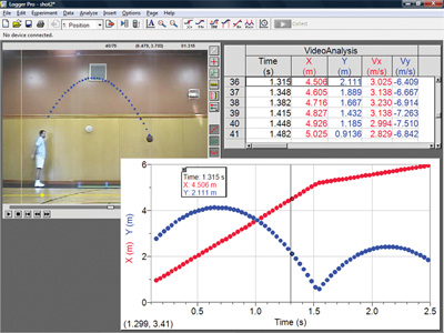 |
 |
|---|---|
Logger Pro screen capture - projectile motion. Logger Pro is probably the most popular program of this type. The earlier version would only take Quicktime format so you had to do a conversion. See Note below. |
Casio Exilim ZR100 is great for high speed photography. As with most high speed cameras the resolution of the video decreases drastically with increasing speed. |
Notes:
iPhone 6 and 6 Plus: these have become popular with students for physics EEIs. Have a look at a simple rebound experiment at 240 fps in this clip by Year 11 Physics student Cassidy Edwards from MBC.
Logger Pro: The newest program takes most popular formats. It costs about $300 for a site licence and can then be placed on the school server or students can install it on their laptops and take it home to use. Also, students can Bluetooth videos from their iPhone and these work fine in Logger Pro.
Tracker: A very popular video analysis program is "Tracker - Video Analysis" which is free. It can import video and export to Excel.
UNIT 3.2 Electromagnetism
Loudspeaker Microphone
Here's a great EEI idea particularly if you are into rock music. Two essential devices in amplified music are the microphone and the loudspeaker. They are somewhat similar: moving-coil microphones use the same principle as in a loudspeaker, only reversed. Microphones have a small movable coil positioned around a cylindrical permanent magnet and attached to a diaphragm (the cone). When sound waves strike the microphone, the coil moves and a electrical signal is induced. In a loudspeaker the electrical current moves the coil and cone and pushes out sound waves. So a loudspeaker can function as a microphone. US scientist Alexander Graham Bell - Professor of Vocal Physiology at the University of Boston - made a fortune from his patent on this idea (Patent 174, 465, 1876; the most successful patent ever).
 |
 |
With two speakers facing each other the sound from the speaker on the left travels through the air as a longitudinal wave and is picked up by the speaker on the right acting as a microphone. |
Yamaha Subkick speaker. About $549 in Australia |
The large diaphragm of a 'speaker' microphone means it can pick up the low frequencies so much better than a conventional microphone. This means it would be great to use when recording a kick drum or bass guitar. Sound recording engineers have been using this trick for years, and Yamaha has made a commercial speaker microphone called the Subkick for this very purpose. But microphones also have to respond to high frequencies so a low mass cone is also important so that it can be accelerated quickly, allowing for fast changes in motion.
The attenuation (energy losses) of sound in air is due to several factors including viscous, thermal and rotational losses (∝f2); and vibrational relaxation of gas molecules. The attenuation of sound depends on temperature, water-vapour content and frequency.
A good EEI would be to set up two speakers facing each other and using one as a speaker that makes the air vibrate in front of it and the other as a microphone picking up the vibrations. That is, they are 'coupled' by the air in between. If you connected them both up to a CRO and fed an audio signal from a frequency generator into the loudspeaker and measured the output of the other speaker you could assess how well the signal was reproduced. Is the quality of reproduction dependent on frequency, loudness, distance apart, diameter of cone, temperature, humidity? What other factor could you assess? How do you define 'quality'?
Resonance in an RLC circuit
A RLC circuit is an electrical circuit consisting of a resistor (R), an inductor (L), and a capacitor (C), connected in series or in parallel. They are used in the tuning circuit for radios for instance.
 |
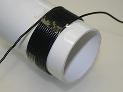 |
RLC series schematic |
A simple coil can be used as the inductor. |
The energy oscillates back and forth between the capacitor and the inductor until internal resistance makes the oscillations die out. In most applications an alternating current is applied, driving continuous oscillations. If these are at the natural oscillatory frequency, resonance will occur. Introducing the resistor increases the decay time of these oscillations, and reduces the peak resonant frequency.
An interesting EEI on this relationship was undertaken by Year 12 Physics student Alex Muirhead from Ormiston College, near Brisbane. Alex proposed that as the AC function generator powering the circuit reaches frequencies near the calculated resonant frequency of the circuit, the impedance of the circuit will reach a minimum.
He prepared his own inductors by winding enamelled copper wire around 70 mm diameter PVC pipe to produce a coil with an inductance of about 300 microhenry (μH). He connected this in series with capacitor and variable resistor across the outputs of a function generator. By comparing the voltage across the resistor with the voltage across the inductor using a digital oscilloscope, the point at which the voltage peaked in the resistor and at which the phase shift was zero gave the resonant frequency. In the graphs below Alex calculated the voltage across the resistor as a percentage of the input voltage from the function generator. They were for circuits using the same coil and 100nF capacitor but with different resistors.
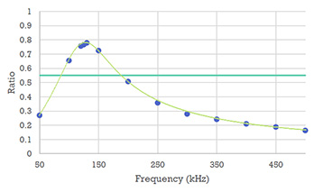 |
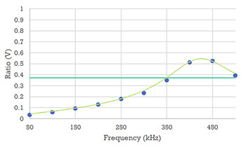 |
Figure 1: For a 10Ω resistor the voltage peak appears around 125 kHz. |
Figure 2: Voltage as a function of frequency using a 50Ω resistor. The peak seems to be at about 425 kHz. |
The "sharpness" of these voltage peaks appears to be related to both the size of the resistor and the capacitor in the circuit. The smaller 10ω resistor and the larger 100nF capacitor both produce sharper peaks than their counter-parts, with the circuit containing both (1.3.3) being noticeably sharper than the rest. The frequency around which these peaks form could be suspected as being the resonant frequency of the circuit.
This made a fabulous EEI and one that I enjoyed reading (and trying to understand the complexities of the problems encountered and solutions). If you are planning a career in physics or electrical engineering this is one prac you will do at university. You would most certainly have to know about it if you were to become a radio and telecommunications specialist.
Resonance and efficiency of induction
Another investigation that maybe of interest follows on from the one above. Alex asked the question: does resonance allow for a greater efficiency of induction? He compared resonant induction with standard induction in a pair of coils by building two circuits, a master and a slave. The master was an RL circuit connected to the signal generator and the slave was an RLC circuit powered by magnetic flux generated from the master. He argued that as the active circuit inducting power into the passive circuit reaches frequencies near the estimated resonant frequency of the passive circuit, the impedance of the passive circuit would be at a minimum, allowing for the most efficient energy transfer across the inductance gap. He attempted to confirm this by finding the conditions under which a peak of voltage formed in the passive circuit, and whether the energy being transferred was at a factor greater than ordinary induction, and whether drop-off was the same.
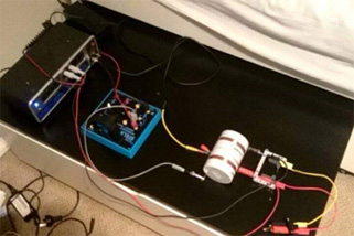 |
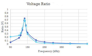 |
| Alex's setup with the master and slave side-by-side. He used 70 mm PVC pipe and enamelled copper wire. | The peak voltage in the slave was at the resonant frequency of the master - in this case 125 kHz for the 10Ω resistor and 100 nF capacitor 'master'circuit. |
The major findings of his investigation suggested that resonant induction is more than 1000 times more efficient than normal induction at the same frequency (thus supporting his hypothesis). However, the drop-off rate between resonant and non-resonant circuits differs, contrary to his hypothesis. There is ample opportunity in such an EEI to propose and test various modifications to the setup - and which would provide an even richer set of data.
Flashing LED - what factors affect flashing rate?
You've no doubt seen the flashing lights on Christmas trees, or the flashing tail lights on bikes, or even a music metronome based on flashing lights. They are all made up of light emitting diodes and an investigation of how they are controlled could make a worthwhile EEI, particularly a guided design one for Year 11. HOD Science at Ormiston College, Brisbane, Paul Dhu has allowed this for his Year 11 class. He said:
"The main prac they do is to construct a flashing LED or simple metronome, and then change the values of the resistors and or capacitors to test the changes in frequency and length if flash. Some students have then backed this data up with simulation data from Yenka (free for home use outside school hours), including graphs of current flow through various parts of their circuits (LED, capacitor, resistor)."
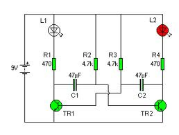
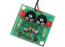
Yenka is a new generation of educational modelling tools from Crocodile Clips and can be used free by students at home. Schools have to subscribe if they want to use it for classwork. Have a look at the Science section at yenka.com. In the physics section there are simulations for "Flashing LEDs" and "Flashing bike lights" (the latter involves the use of 555 timers). Paul Dhu says "If they're in Yr11, I would steer them away from circuits that use the 555 timer IC chip, but depends on you of course."
A Simple AC Generator
The discovery that the motion of a magnet past a coil of wire produces an
electric current was made by Michael Faraday 160 years ago. Since then this
relationship has been investigated by countless scientists, engineers and
students. You would think that there is nothing left to discover but some
interesting things are always thrown up by investigators. Electromagnetic
induction makes a good EEI, partly because it can be done simply and partly
because interesting data gives you lots to talk about. Physics teacher at
Urangan State High School, Queensland, Australia, Alan Whyborn describes an
experiment that could be the basis of an EEI.
He took a standard air cored solenoid (basically a coil of wire wrapped on a plastic tube; very common in physics labs) and suspended a magnet on a piece of string near the end of the solenoid (see photo below):
I suspended a rare earth magnet outside the coil with cotton in such a way that I could wind the cotton up, release the magnet allowing it to spin, and record the results with a datalogger (set on highest sample rate). The data clearly showed that as the magnet spun faster, the voltage increased. We were then able to measure the peak voltage and period at a variety of times (a range of rotational speeds). The easiest way to do that was to "select" two periods and do a sine curve fit (which provides amplitude and period).
Doing this at six different areas of the
data (from near slowest to fastest rotation) and creating a graph of voltage vs
frequency gave the expected linear relationship with a very high
correlation." Maybe you'd like to take this further.
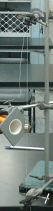 |
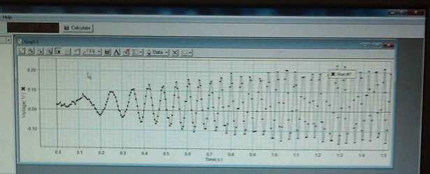 |
| The setup | A screen capture of the data. You can see how the period of rotation gets smaller from left to right and how the corresponding voltage increases. |
Electromagnet cores and magnetic field strength
In Junior Science you probably made an electromagnet by wrapping wire around a tube and connecting it to the laboratory power supply. When you put a nail inside it you could pick up paper clips. The question is: why do you need a metal core to make it work as an electromagnet? Would a steel bolt work better than a bunch of nails lined up side-by-side? Do laminated strips of metal (see below) work better than a solid piece of steel.
 |
 |
Electromagnet being used at a scrap metal yard. What is the core made up of? |
A transformer taken apart. Note that dozens of E-shaped pieces of metal are used to go inside the coil rather than just a solid piece. The transformer is said to have a "laminated" core. |
Stephen Pinel, Head of Science at Proserpine State High School, Queensland said: "I had a group of students last year who investigated the effect of different cores in an electromagnet, measuring the magnetic field strength using a Hall Effect Device, which is $5.75 at Jaycar. Got some great results, but they did go through a couple, and made a bit of smoke at times (which just added to the general excitement)."
 |
Hall Effect Sensor - a miniature sensor to accurately track extremely small changes in magnetic flux density. (Jaycar) |
Electromagnetic Strength
Another thing you could investigate is the magnetic field strength of a solenoid. The photo below may give you some ideas. A permanent magnet is suspended from a digital force meter.
 |
Here's Alex Camp's setup for his investigation into the force acting on a bar magnet inside a solenoid. Alex is a Yr 12 Physics student at Churchie, Brisbane. (Alex Camp) |
Electromagnetic Shielding
Electronic equipment sometimes requires isolation from external magnetic fields otherwise it may malfunction and cause accidents (eg a plane fall out of the sky). Humans too are susceptible to magnetic fields. For instance, in an Magnetic Resonance Imaging (MRI) machine used for diagnostic testing, the patient is subjected to a very large magnetic field (1-3 T). However, the operator doesn't want to experience the field as it can cause health effects: dizziness, nausea and taste sensations (particularly if he/she does a lot of tests per day. People outside the MRI room (nurses, doctors, office staff and the public) need to be protected too. Passive shielding is done with steel plates either as part of the magnet gantry or attached to the walls, ceiling and floor of the examination room.
 |
 |
The Siemens Magnetom Verio 3T Magnetic Resonance Imagining machine at one of Queensland X-Ray's clinics in Brisbane. As the name suggests, the magnetic field strength inside the machine is 3 Tesla (permitted maximum is 4T). The stray field from such a machine is quite low (perhaps as low as 0.5mT) because it is well shielded. |
Workmen fitting steel plates to a room before the installation of an MRI machine. This will shield people in the next room from stray magnetic fields. Would they need to fit plates on to the ceiling (which has steel framing) or to the floor (which has steel mesh reinforcing)? |
Why steel? Is it because it is effective or because it is cheap? Is there anything better? For static (stationary) or slowly varying magnetic fields (below about 100 kHz) shields made of high magnetic permeability metal alloys are generally used. Shielding materials don't block the magnetic field, but rather draw the field into themselves, providing a path for the magnetic field lines around the shielded object. The effectiveness of this type of shielding depends on the material's permeability, which generally drops off at both very low magnetic field strengths and at high field strengths where the material becomes saturated. There is another type of shielding - Active Shielding - which uses a second coil external to the windings of the main magnetic field. The field generated by this secondary coil is oriented to oppose the main field and reduce its spread. This is also used for MRIs in addition to passive shielding.
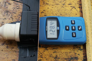 |
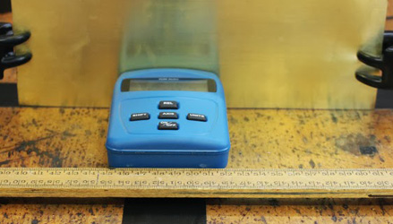 |
| James Stewart's group at Villanova College, Brisbane, used a power adapter as the source of the magnetic field. It is shown here with a sheet of aluminium interspersed. The reading of 128.4 is in microtesla. | Here's a setup James Stewart's group used at Villanova College. They also measured the shielding of a big AC laboratory power supply which has a big transformer inside it. |
A successful EEI can be built around investigating the passive shielding effect of different thicknesses of different materials, perhaps using a Hall Effect device as a sensor. However, it is no good just testing a few materials and saying which is the best; you need to hypothesise which would be best and justify your choice by reference to physics facts and principles. If you are not using a Hall Effect IC (or a Gauss Meter - shown above) to measure the field, you will have to design a method that makes sense - eg picking up unmagnetised paperclips. This may seem easy but will require a lot of thought. A fabulous EEI if it comes off. And so useful. One thing I'd like to know is why a steel gauze Bunsen Burner mat is just as good as a sheet of steel for shielding. Wouldn't the magnetic field get through the holes in the gauze?
Electromagnets - factors influencing their performance.
The shape of an electromagnet coil seems likley to affect its performance. For instance - a short coil with lots of turns of wire would seem better than a long coil (a 'solenoid') even with the same number of turns. But how does the diameter affect the strength of the magnetic field, or the electrical current for that matter?
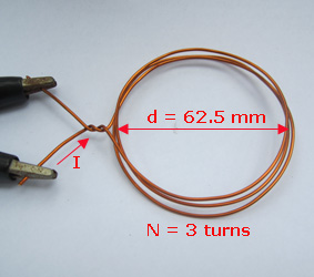 |
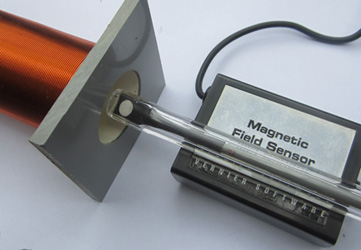 |
The magnetic field strength at the centre of this short coil is given by B = πkI/r where r = radius. For 3 turns the B value would be multiplied by N = 3 turns. |
A Vernier Hall Effect probe being used to measure the magnetic field strength at the centre of this solenoid's end. The formula is B = 2πkIN/L. The solenoid in the photo has a diameter of 34 mm, a length of 140 mm and 300 turns. |
Electromagnets - near fields and far fields
One of the most intriguing things you can measure about the magnetic field is how it decreases with distance. A good EEI can be made from the measurement of field strength with distance from an alternating current device such as a lab power supply. You could equally use any domestic appliance to give your investigation a real-world context. Things like a bar heater, a hairdryer, a toaster, a clock would all work but a lab power supply with a constant output (say 2V across a 50 ohm load resistor) might be worth a shot.
I approached colleague Dr Donald Polvani, former Advisory Engineer, Northrop Grumman Corp. and former Adjunct Faculty, Physics, Anne Arundel Community College, Maryland, USA - a renowned expert in this field - for suggestions about this EEI. He said that where it becomes fascinating is that a changing electromagnetic field (around an AC source) has three magnetic field zones associated with it. Dr Polvani suggested that a good reference was the text by John David Jackson, "Classical Electrodynamics", John Wiley, NY, Section 9.1, pp. 268-271 (1962). The latest version of this graduate level text is the third edition published in 1998. However, it turns out that the original (1962) version is available for free download. The zones (mentioned in Jackson) are:
For a Australian 50Hz AC supply the wavelength is c/f = 3 x 10⁸ms-1/50Hz = 6000 kilometres, thus any lab-based experiment has to be in the Near Zone or what you could call the "Ultra-near Zone". Dr Polvani suggests that in order to measure the expected magnetic dipole 1/r3 spatial fall-off for r >> d, either the measurements should be continued for several metres away from the source, or a smaller source should be used. He said "Consider making a small rectangular coil source fed by a low voltage transformer and in series with a variable power resistor. This way both the dimensions of the source and the current through it can be directly controlled and measured."
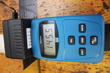 |
 |
James Stuart's group at Villanova College used a power adapter for the magnetic field. The reading is in microtesla. Dr Polvani suggests a home-made coil whose dimensions are able to be measured. |
The students also measured the field at different diatances away from the source. They did this not only straight out from it but to the sides as well. The reading at this position was 14.7μT. |
My thanks to James Stuart for his data. If you do this EEI be prepared to do a lot of work on near and far field theory. There's an A+ awaiting if you can get a handle on it.
Triboelectric charge as a function of work done
A student
(Sarah - below) said she was fascinated by the triboelectrification of plastic rods after seeing a demonstration of the effect of charge on a stream of water. Triboelectrification is producing an electric charge by rubbing a rod on rabbit fur, silk, wool and so on.
She wondered if there was a relationship between the work done in rubbing them and the quantity of charge developed. This seemed interesting but I warned her that there were many things to control (humidity, temperature, the type of fur, the method striking the rods and how the charged was to be measured). Despite my hope that she would abandon this as an EEI, she insisted - so good luck to her.
The student is Sarah in my Year 12 Physics class at Moreton Bay College. The design was all hers and she ran into may challenges. Ultimately, she ended up measuring the quantity of charge by the angle of the vane in an electrometer. We didn't have anything too flash so she had to make do with a simple one with an aluminium vane. As a second variable she tried the type of rod (perspex). The problem was that as she didn't do chemistry it was hard to describe the bonding differences between hard rubber and perspex, and the ease of electrification this may result in. She seemed to get a good relationship between angle (charge) and (number of strokes) work done. The different rods gave a noticable difference. Several weeks on the internet was needed to finish her project off. I'm not sure that I would advise this unless you like a design and control challenge. Way to go Sarah!
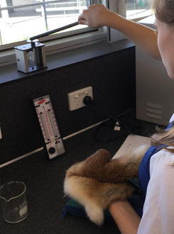 |
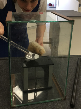 |
| The Wet and Dry Bulb Hygrometer is there to ensure humidity is controlled. I assured her that all furs came from the same cats. Or was that rabbits? | Sarah had to control how she put the rod on the cap of the electrometer. So many errors to watch out for. The fish tank was to stop the breeze from the airconditioner. |
Transistors and temperature
You don't see many Senior Physics EEIs based around transistors. I think it is because the theory just gets too hard. But I have a suggestion below for those who are keen on electronics. It is about how the collector current changes with temperature.
In school physics, the usual experiment involving transistors is to vary the base voltage and measure the change in voltage across the load resistor connected to the collector. This is just the voltage gain. Students also do current gain (current amplification) but that's about all. This doesn't make for a very rewarding EEI. My suggestion is based on the work of Professor Michael Sturge and Song Bac Toh from Dartmouth College, New Hampshire, USA ["An experiment to demonstrate the canonical distribution". Am. J. Phys. 67 (12), Dec 1999, p1129-1131]. They set up a simple transistor circuit and varied the base voltage and noted the collector current. However, they did this at three widely spaced temperatures (200K, 295K and 368K). Song Bac Toh is now with Cisco Systems in the US and he gave me some clues (2016) about his experiment - which I have tried, succesfully.
My circuit diagram is below. You can work out the base voltage used and the collector current from the graph. They used three temperatures: a dry ice-propanol bath at 200K, room temperature ~298K, and an oil bath immersed in boiling water at 368K, and placed the transistor in the liquid (nothing else).
Circuit for this EEI. |
Plots of log10 Ic against V are linear. |
Why does this happen? The thermal energy increases the motion of electrons in an n-p-n transistor and helps them overcome the junction barrier. An electron has a certain probability of occupying a state above the barrier but if heated it can cross the barrier and reach the collector, contributing to what is called the "diffusion current" from emitter to collector.
Michael and Songtoh then did an Arrhenius plot of log10(IcT3/2) against 1000/T:
The graph is linear. |
Scattering of light in milky water #1 - attenuation of different wavelengths with depth
Dr Stephen Hughes from Queensland University of Technology, suggested a possible EEI investigation about the scattering of light in a beaker of milky water. His own work into how a Blood Moon originates prompted a discussion about shining a white LED torch into the side of a beaker of water to which a few drops of milk has been added.
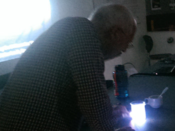 |
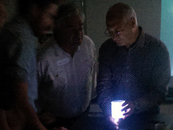 |
| Dr Stephen Hughes demonstrating scattering of light in milky water at an EEI Workshop at Moreton Bay College. | He recommends a white LED torch with a single beam. That's Steve Smith from Yeronga State High looking on. |
As the torch is moved down the side of the beaker the beam of light appears more yellow as it has to travel through more and more of the cloudy liquid to reach your eye. He suggested photographing the view from above (see photos) and analysing the image for RGB levels. Stephen suggested using the photo analysis program "Imagej" but I found some of the other on-line apps easier to use. For the data below I just used Martin Krzywinski's "Image Color Summarizer" - mkweb.bcgsc.ca/color_summarizer/. The colour doesn't appear much different to the human eye but a difference there is.
 |
 |
 |
 |
20 cm deep |
40 cm deep |
60 cm deep |
80 cm deep |
Then as more and more scattering takes place as the depth increases, the loss of blue light through scattering means that the proportion of red/yellow in the transmitted light increases. That seems true in the photos above, but what the relationship is not certain from the photos. That would make a great EEI.
Light attenuation in cloudy water #2 - effect of depth
In World War 2 the public were asked by the Australian Army Inventions Directorate to suggest new ways of detecting submarines - and were promised a reward if it worked. Several thousand suggestions came in and they were checked by Dr Kerr Grant, Professor of Physics at the University of Adelaide. A common suggestion was to use an underwater searchlight. He was most scathing and said "the attenuation of light in sea water makes this suggestion nonsense".
The attenuation coefficient (mu μ) characterizes how easily a fluid (such as water) can be penetrated by a beam of light, sound, particles, or other energy or matter. A large attenuation coefficient means that the beam is quickly "attenuated" (weakened) as it passes through the medium, and a small attenuation coefficient means that the medium is relatively transparent to the beam. To make water attenuate a beam of light you can add a few drops of milk (a few drops in 500 mL). The fat globules cause "Rayleigh Scattering" so the light is scattered as it passes through the water. This suggests a good EEI. Shine a beam of light from a laser or a white LED torch through a milky solution and measure the intensity (transmittance) of the beam using a light meter. I tried an Arduino with a light sensor and it worked well.
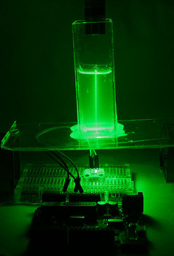 |
I made up a cell from four microscope slides glued (epoxy, eg Araldite) together along their long edges to make a hollow box, and then glued it to the lid of a CD case. The green laser shines through the milky water on to a photocell connected to an Arduino. The Arduino 'sketch'program reads the brightness of the light and return a value between 0 and 1023. |
Next, change the path length of the milky water and take more readings. I did this by adding the milky water to the cell 1 cm at a time and measured the resulting transmittance. I also measured the initial transmittance using an empty cell. I 'normalised' the transmittance by calculating it as a fraction of the initial transmittance (T (normalised) = T/Ti). The behaviour of the light should decay according to the Beer-Lambert Law: T = Ti e-μL, where L is the path length and μ (mu) is the attenuation (or extinction) coefficient. The term extinction coefficient is an older one.
Hence T/Ti = e-μL. If you plot T/Ti (y-axis) vs path length L you should get a curve (see below). Take natural logs of both sides: ln (T/Ti) = -μL, so if you now plot -ln(T/Ti) vs L you should get a straight line (y = mx) with the slope being the attenuation coefficient. You could increase the concentration of milk and you should get a bigger attenuation coefficient.
 |
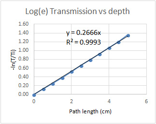 |
| My results for a red laser. You get a curve but the trendline suggests a exponential relationship. | Negative log(e) graph gives a straight line with a slope of 0.2666 cm-1 - which is the attenuation coefficient μ (mu). |
Light attenuation in cloudy water #3 - effect of wavelength
In the above suggestion the light path was changed (the manipulated variable) and the wavelength of the light was kept constant. A good EEI can be made by doing the above experiment but varying the wavelength as well. Lasers come in many different wavelengths but the common ones are red (635 nm), green (532 nm) and blue (473 nm).
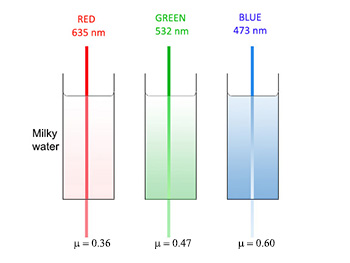 |
Blue laser light is scattered the most as it passes through milky water. The higher the attenuation coefficient (μ) the greater the scattering. Blue has a μ of 0.60 which is higher than red (μ = 0.36). These values were for one experiment and depend on how much milk is added. |
I repeated the above experiment using these three lasers colours and fresh milk, and worked out the attenuation coefficient for each (as in EEI #2 above). In theory the amount of scattering is proportional to the 4th power of frequency. As frequency is proportional to the reciprocal of wavelength we can say that the amount of scattering is proportional to 1/λ4, or λ-4. The amount of scattering can be characterised by the attenuation coefficient (μ). If you plot μ (y-axis) vs wavelength you should get a curve. Use Excel's power function to suggest a value. Ideally it would be -4 but you could plot u vs wavelength raised to the power of -4 you should get a straight line. I did an the R2 value of 1.00 suggests that μ ∝ λ-4 is a good fit. Over to you.
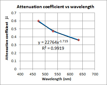 |
 |
This is a 'power'curve and Excel suggests it is to the power of -1.715 whereas theory suggests -4. |
When the data are plotted against the wavelength to the power of -4 a straight line results. This 'linearisation'of the first graph proves that the attenuation coefficient is indeed proportional to the wavelength raised to the power of -4. |
Light attenuation in cloudy water #4 - the half-value layer (HVL)
Engineers need to know the attenuation coefficients for various substances based on the type of radiant energy or matter passing through. This helps them decide how much protection is needed for safety from potential harmful radiation (eg alpha, beta, gamma radiation, sound, heat and so on). Instead of using attenuation coefficients they use a more easily understood property called the half-value layer (HVL). It is the thickness (path length) of a medium that will reduced the transmission (or intensity) to half the initial value. On the graph below, to get a transmission of 0.50 you need a depth of 2.4 cm.
If you do the full experiment and calculate the attenuation coefficient you can then use the decay equation T = Ti e-uL and let T = Ti/2, you get Ti/2 = Ti e-uL. Cancel out the Ti and take the natural log of both sides and you get 0.693 = μLHV. If, for example, you found the attenuation coefficient to be 0.27cm-1 for red light then LHV = 2.4 cm. This agrees with the graph below.
 |
| The Half Value Layer can be read off a graph of Normalised Transmission vs Path Length. In the case above, the HVL is 2.6 cm. That means if you filled the cell to 2.6 cm depth of milky water the transmission reading would be half that of an empty cell. |
Light attenuation in cloudy water #5 - transmission vs scattering
As shown above when light is passed through a suspension it is attenuated. That is, the transmitted light is not as intense as the incident light. This happens for small colloidal particles in suspension such as milk protein. The process shown in the EEIs above is called 'turbidimetry': it is the measurement of the degree of attenuation of a radiant beam incident on particles suspended in a medium, the measurement being made in the directly transmitted beam. But light is also scattered in all directions as it passes through the suspension. You can also measure the 'scattered light' by a technique called 'nephelometry': the measurement of the light scattered by suspended particles, the measurement usually being made perpendicularly to the incident beam.
Turbidimetry or nephelometry may be useful for the measurement of precipitates formed by the interaction of very dilute solutions of reagents (great for a Chemistry EEI), or other particulate matter, such as suspensions of bacterial cells.
A fabulous EEI would be to examine the light scattered (by Rayleigh scattering) through the sides of the glass cell. You could even do it in a beaker as in EEI #1. I just sticky taped a light dependent resistor (LDR) on the side of a cell, and taped another LDR underneath it. I connected the wires to the analog inputs of an Arduino board (each in series with a 100 ohm resistor) and used a 'sketch' that read the outputs across the LDRs. It is very simple and worked well. The circuit diagram and the sketch is here if you want it.
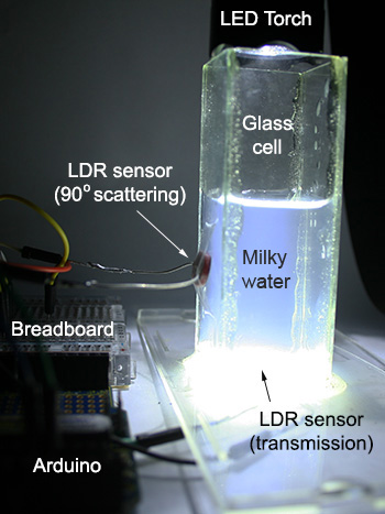 |
I used a LED torch instead of a coloured laser. |
I placed 25 mL water in my glass cell and took LDR reading for transmission (turbidimetry), and scattering (nephelometry) as I added drops of milk. Turbidity is expected to follow a logarithmic relationship with concentration: -log10(I/Io) = kbC where k = the turbidity constant, b = path length, C = concentration. So if you plot -log10(I/Io) vs concentration you should get a straight line.
The relationship between scattering (90°) and concentration is linear: if you double the number of suspended particles you get double the scattering. The relationship is Is = KsIoC where Is is the scattered intensity, Io = the incident intensity, Ks = scattering constant, and C = concentration. Have a look at my rough graphs:
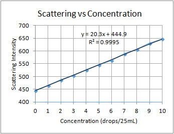 |
|
Turbidity graph: plotting log of transmission vs concentration linearises the graph and confirms a logarithmic relationship: y = 0.0023x + 0.0003, R2 = 0.9964 |
Scattering graph is linear (hooray!). |
Surface Tension of Water - Tate's Law
You've seen water bugs standing on the surface of water. We can't - so how
come they can? The property of liquids - surface tension - is critical in all of
our lives from the control of it in our bloodstream to large scale engineering
applications. Year 12 student at Villanova College, Coorparoo, Brisbane,
David Thompson chose to investigate this phenomenon for his EEI in consultation
with his Physics teacher. David wrote:
"This experiment aimed at investigating the surface tension of water at different temperatures and with detergent. It was thought that an increase in temperature would result in a linear decrease in surface tension and that the addition of detergent would reduce the surface tension of plain water to about a third of its strength. The surface tension was measured using a suitable needle and dripping a liquid from it, inspired by Italian physicist Gianino Concetto".
He relied on Tate's Law that says when a drop falls from an orifice (like a syringe needle) pdG = mg (where tau (G) is the surface tension). The rest you can find elsewhere. You have to ask: how do I measure the mass of a single drop and the diameter of the needle? At 293K David was getting drops with a mass of 1.48 x 10⁻⁵ kg and at 313K 1.36 x 10⁻⁵ kg . Surface tension was about 60 mN m-1. Over to you.
 |
 |
 |
| A water droplet about to fall | Syringe | Oil droplet. Photos by David Thompson. |
Capillary Action in a Water Wedge
Leonardo da Vinci must be considered as the discoverer of capillary phenomena, but the first accurate observations of the capillary action of water between glass plates were made by Francis Hawksbee in 1709. In his textbook he noted that the height of its ascent varied according to the distance apart of the glass "planes":
Physico-Mechanical Experiments, London, 1709, p 140. |
In 1712 he wrote a paper in the Philosophical Transactions of the Royal Society of London (V 27, p 539) where he ascribed the action to an attraction between the glass and the liquid. From his data he concluded it was a hyperbolic relationship. From then on physics texts routinely included his experiment. An early example shown below comes from an 1860 American textbook (left). My attempt to repeat his experiment is on the right.
 |
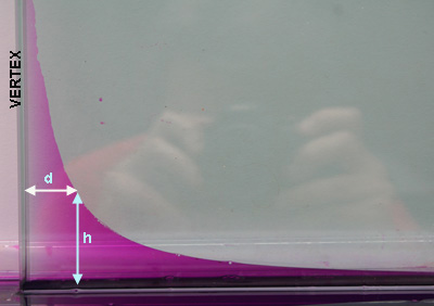 |
Physicist and author Benjamin Silliman, in 1860, wrote "When capillary action causes liquid to rise between two plates forming a narrow wedge, the upper surface of the liquid follows a hyperbolic shape." Principal of Physics, or Natural Philosophy, 2ne ed. (Ivison, Blakeman, Taylor & Co., NY, 1860, p194). |
My experiment: A thin film of water trapped between a wedge formed by two sheets of glass at small angles to each other. The water is coloured with some potassium permanganate (Condy's Crystals) although food colouring would also do. Be careful: you don't want to stain mum's kitchen bench. |
In your studies of solid geometry you would have learnt that the hyperbola is made by slicing a cone with a plane perpendicular to its base. In physics it appears when one property of a system is proportional to the reciprocal of another property, ie y ∝ 1/x. The analysis shows that the height to which the water drawn up by capillary attraction is proportional to the reciprocal of the distance from the vertex of the wedge, and hence the hyperbolic shape of the surface of the water.
A good EEI would be to investigate this capillary behaviour of water. I used two pieces of window (louvre) glass clipped at the left with a bulldog clip, and a piece of wire holding the glass apart at the right. To get the data I just enlarged the photo and printed it off on some A4 graph paper. I was thinking of enlarging it to A3 size in a photocopier but it was during the school holidays and I wasn't that keen.
You would have to do more than just plot your data. You would of course plot y vs 1/x to see if it is a straight line but this is not enough for an "A". You would need to do triplicates for each diameter of wire, and try to explain any differences. Then you could change the diameter of the wire to give you say 5 "treatments". The theory is easily found in most physics texts or on the web. Now you'd really have some explaining to do.
The World's Simplest Motor
The "Homopolar Motor" has to be the world's simplest. It was invented in 1821 by
Michael Faraday. You'll find ones on You Tube purporting to be simple but
not as cool as the one below. "How does it work?" was set for the 2009 IYPT
competition in China. Briefly, (and I don't want to give you too much help) when
you touch the wire to the side of the magnet, you complete an electric circuit.
Current flows out of the battery, down the screw, s******* through the magnet to
the wire, and through the wire to the other end of the battery. The magnetic
field from the magnet is oriented through its **** faces, so it is ******** to
the magnet's axis of symmetry. Electric current flows through the magnet (on
average) in the direction from the centre of the magnet to the ****, so it flows
in the ****** direction, perpendicular to the magnet's axis of symmetry
 |
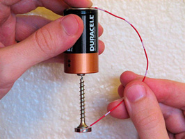 |
Roof colours - white vs
black
Nobel laureate Steven Chu, former
professor of physics at the University of California and nowU.S. Energy
Secretary in President Obama's administration says "white
paint is what's needed to fix global warming". However, Steven Chu said, even if
we paint every roof white, "there was no silver bullet for tackling climate
change, and said a range of measures should be introduced, including painting
flat roofs white. Making roads and roofs a paler color could have the equivalent
effect of taking every car in the world off the road for 11 years." That sounds
like an ideal EEI.
One Australian company sells just the thing: White
Roof Shield is a white coating which reflects 80% of the sun's radiation.
They say it "helps reduce interior cooling loads of air conditioned structures,
resulting in savings of both energy and money. Even buildings without air
conditioning stay cooler because roof surface temperatures are significantly
reduced". Put some roofs of different amounts of whiteness in the sun for some
time and measure the temperature of something underneath (maybe air, water).
Maybe a heating curve is best. May need more than three trials, and what's the
best way to produce this (mixing black and white paint proportionally, black
masking tape etc). What about flat paint vs satin vs glossy?
 |
 |
Home
Insulation - is thicker better?
Ceiling insulation is one way of
improving the energy efficiency of a home. Insulation materials such as
polyester, fibreglass or wool "batts", metal foil and shredded newspaper are
just some of the ways it can be done. In 2010 the Australian Government
subsidized the installation of batts and foil in 550000 homes at a cost of $2.45
billion. Many were installed improperly and in some case fires and death
occurred. The research question that could be useful for a Senior Physics EEI is
what factors affect the thermal insulation property of a material?
There is a
great temptation to compare the various materials to see which performs best;
but you have to ask "what variables are you considering?". Such a comparison may
be okay for a Junior Science project or EEI but it is very problematical for a
Senior Physics EEI. Presumably you would have different building materials to
test but the question is: what is the manipulated variable. If it is just "type
of material" then on what basis are you comparing them? You could have variable
R-values but you would need to keep all other variables constant (thickness,
surface area, heat source, time).
My suggestion is to investigate varying thickness of a single insulating
material. That way there would be some physical quantity to analyse other than
R-value (which is merely the result of an experimental determination anyway).
The last thing you want is the temperature inside the house for a bunch
of building materials without any physics theory behind why they have different thermal
conductivity other than "they just do". That is, what is their relationship to each
other? This is a physics EEI and physics principles, theories and concepts must
be at the forefront of any investigation. Otherwise, I think you would find difficulty in being able to
address the the criterion (Queensland Syllabus IP3):
"identify relationships between patterns, trends, errors and anomalies"
when
there is no theoretical scientific relationship proposed in the hypothesis. This
also applies to criterion EC1: "analysis and evaluation of complex scientific
interrelationships". Varying the thickness avoids this.
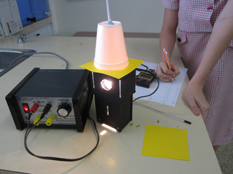 |
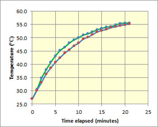 |
 |
| Here's a suggestion: use a light-box kit to provide the
source of heat. I put the insulating material (yellow cardboard) on top
and then a polystyrene cup with a thermometer stuck through it to record
the air temperature inside the cup (the "home"). Worked like a charm - and
so simple. As a bonus, you could even look at a second variable - that of
the temperature of the heat source (try 12V, 10V, 8V....). |
My graph showed that the single layer of card (top line)
allowed the temperature to rise quicker than for two pieces of card
(bottom line) but after 25 minutes they were both the same. Hmmm - how to
explain that? This is a rich source of data. What would three pieces of
card show? |
I also tried six layers of paper towel but the
temperature shot up very quickly at first (6 degrees in 1 minute). Why was
that? I think hot air made its way through the paper. But 6mm expanded
polystyrene foam was no better. What a great source
of data to analyse. Do it well and I'd have to get an A+. |
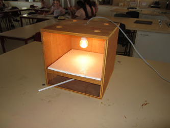 |
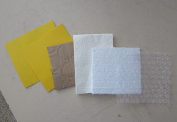 |
| Another idea is a wooden box with a 240V lightbulb as the source of heat. There is a piece of wood that fits on the front. In this photo, a sheet of 8mm polystyrene is being tested. | Here's a few things you could try. But remember, you are not comparing different materials unless you can establish some physical relationship between them in terms of their insulating ability. Comparing their thickness makes for a good EEI (1 layer, 2 layers, 3 layers). |
Some teachers have used this idea in the context of "sustainability". Students investigated the effect of thickness of more natural construction materials such as clay (roll out thin layers of terra cotta clay from the Art Department). In this cases you would be looking at wall insulation, not ceiling insulation.
Tennis
Racquet - Sweet and other spots
On the face of the tennis racquet, there are
several points that are important to players; these are the centre of
percussion, the vibration node, the best serving spot, the best returning spot
and the dead spot. A couple of the spots are shown on the diagram below. The
centre of percussion is one of the two "sweet spots" of the racquet. This is
because at the point of impact between the centre of percussion and the ball,
the hand can feel no impact. This is due to the fact that the centre of
percussion is located near the centre of the face of the racquet. You can
easily find out what all this means and about the other sweet spot.
A good EEI
would be to test the 'coefficient of restitution' (ratio of bounce height to
drop height) of different parts of the face. Perhaps clamp the racquet in a vice
and drop a tennis ball on different position of the face and noting bounce
height as a fraction of drop height. Does drop height affect the coefficient of
restitution? Is the type of ball important? Does a temperature change shift the
sweet spots? Are new racquets better than old? Is aluminium better than
graphite? Does string tension play any part? The possibilities are endless. The
photos of professional players show that the serving spot is high and the return
spot is low. Note: Brad Barker from San Sisto College has listed "Physics of Sport
EEIs" that have worked at his school. Click here to download.
 |
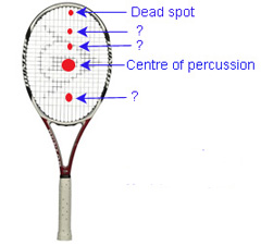 |
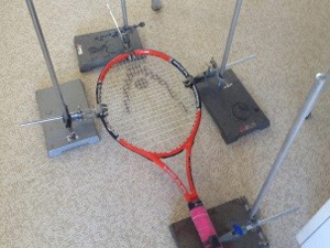 |
Perfect serving spot. |
The various 'centres' on a tennis racquet. |
Experimental setup at Moreton Bay College for Year 12 Physics EEI - 2013. |
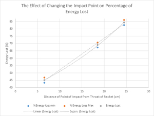 |
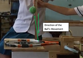 |
| Year 12 student Chelsea Meadows at Mansfield State High School used Logger Pro to analyse data of a tennis ball landing on a tennis racquet. The graph shows the energy lost going across the surface of the racquet from the neck. | Chelsea's photo shows that the ball rebounded at an angle and as you go across the face of the strings the rebound angle changes. My thanks to Chelsea for letting me use her excellent EEI (November 2017). |
Danger inside a hot car
After rescuing 20% more children from locked cars
last summer than the previous year the Royal Automobile Club of Queensland has
urged parents not to leave children locked in cars. The RACQ says that on
a typical Australian summer day, the temperature inside a parked car can be 30°
- 40°C hotter than outside the car. That means that on a 30°C day, the
temperature inside the car could be as high as 70°C and 75% of the temperature
increase occurs within five minutes of closing the car. They also say that
darker-coloured cars can reach a slightly higher temperatures than
lighter-coloured cars (I would have though much higher temperatures); and
that large cars can heat up just as fast as small cars.
The key variables are
obvious for an EEI and having a data logger would be great. But some others
worth considering are the colour of interior trim; having the windows down a
bit, or even fully open; dark vs light colours; big vs small; time of day (angle
of sun); and window tinting. You could even model a car by using painted
soft-drink cans and sealing a thermometer into the hole with Blu-tac. Maybe you
could puncture holes in the side to represent an open window (or vary the number
of holes as a manipulated variable). Oh, the possibilities are endless but and it looks easy but controlling the variables will be
important.
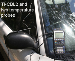

Descent of golf balls down an incline
If
you roll a golf ball down an incline you should note that as the angle increases
so too does the velocity. You could measure time vs. angle; time vs. distance.
Is acceleration uniform? Why do similar looking balls give different results;
perhaps it is to do with their construction (see 2-piece, 3-piece and 4-piece
types below. Maybe it is to do with their dimples or hardness (Novice = long,
soft; Intermediate = very long & soft; Power = straight & very soft; Titleist = extremely long, and so on). Try removal of dimples! Use a light gate at bottom to
measure final velocity; how does this compare with 2 x vav? That's
Melody's hands in the photo below. She's from Moreton Bay College.

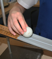
Cars on a ramp - angle and
speed.
If you ride a
skateboard down a hill you know that your speed increases as you go down. This
happens for all sorts of things: riding a toboggan down a sandhill, skiing
down a ski run, letting a shopping trolley go in a carpark, and going downhill
on a bike or roller skates. Even cars get faster if they accidentally roll
down a hill. You can reach dangerous speeds if you have no way of braking or
slowing down. With cars and trucks it may be impossible to stop them and the
consequences can be disastrous.
An EEI could look at factors that
affect the speed of an object as it moves freely down a slope. Knowledge of
these factors may help in the design of sports grounds skateboard bowls, ski
runs, toboggan slides and so on. It could even help road engineers ensure that
road inclines do not create dangerous situations. What could make a good EEI
is to consider the relationship between height of the incline and the final
speed of the car after a certain distance, keeping mass and the surface type
constant. This does make an excellent Year 10 EEI but it also is very suitable
for Year 11, particularly if you choose to look at a second variable (mass).
.jpg) |
| We all know that GPE is converted into KE but is it
100% efficient? By timing the car over the metre you can work out the
final speed assuming constant acceleration. Varying the angle will give
different times. Don't forget to include 0.0 cm height = 0.0 m/s final
speed. You would think you'd get a y ∝
√x relationship but
mine didn't look exactly like that. Plenty to talk about. For 6 cm, 9 cm
and 12 cm ramp heights with a 72g toy car I got final speeds of 70, 124
and 131 cm/s
over the 1 metre.
Efficiency of energy transfer was 42%, 87% and 73% respectively. Hmmm! |
Cars on a ramp - stopping distance of toy cars along the floor due to friction
For sliding friction on an incline, the coefficient of friction μ =
tan θ for constant speed; but for rolling friction it may not be. You could let
a car roll down a ramp on to the horizontal floor and see how long a distance it
takes to stop. How does this vary with the height (which determines the starting
speed) at the bottom of the ramp. It maybe tempting to use a solid ramp but the
join at the bottom may not be smooth and the bump can slow the motion. To get a
smooth run a curved surface could work. I just used some carpet tiles with the
shiny side up.
The question is: where is the friction in a toy car travelling
along a surface: between the axle and the wheels, or the wheels and the road?
You could also look at the effect of the mass of the car and so on. What are the
practical implication for this? Does twice the mass (eg a truck compared to a
car) mean twice the stopping distance? It is tempting to compare the rough
carpet side with the smooth side, or to compare different carpets but the
question is: just how is your "roughness" variable measured. Maybe you could
measure the coefficient of friction of the material first and use that as the
variable. This is certainly not as simple as it looks and may, at first glance
look just like a Year 10 EEI but there is a lot in it and could be good at a
Year 11 level.
 |
The distance d (or displacement s) is easy to measure but how exactly do you measure the change in height h for used in the GPE = mgh formula? I've shown it here as the vertical distance between the centres of gravity at the top and bottom of the ramp. But could that be improved? Can you assume the conversion to KE is 100% efficient to work out the speed at the bottom of the ramp? Would you need to measure the time elapsed to be able to calculate the deceleration of the car along the horizontal (a = (v-u)/t) or could you use v2 = u2 +2as? Is all of the GPE converted to work done in bringing the car to a halt (GPE = mgh = W = Fs = mas)? Whew, so much to think about. |
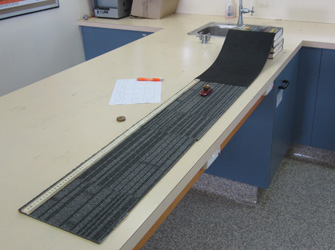 |
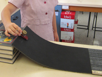 |
| On this rough side of the carpet tile and a starting
height of 4 books (11.8 cm) the car travelled 83.2 cm unloaded but
travelled only 63.2 cm with a 50 g mass Blu-tacked to its hood. |
Still with a starting height of 11. 8 cm but with two 50 g masses on the hood the car travelled just 42.3 cm. Is
distance proportional to mass? |
Using a Smartphone Accelerometer on an inclined plane
The Queensland Studies Authority has an "A" standard sample EEI on their webpage that describes the use of a smartphone in measuring acceleration down an incline. It may provide some good ideas about what you can do - and gives you an indication of what an "A" response could look like. Click here to download.
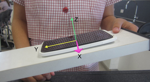 |
3-D accelerometer apps are available free for all phones (Moreton Bay College) |
Rolling friction of a ball
When a ball rolls along a surface it will eventually come to rest.
Because it gradually slows down we say there must be a force opposing its
motion, and we call this force "friction". We can think of friction being
classed as three types: static (not moving), sliding, and rolling. In class, you
will have most likely dealt with static and sliding friction because they is easy
to demonstrate and quantify (slide an object across a bench or down an incline). In
contrast, rolling friction is harder to measure as it is usually much smaller.
If a cylinder or ball is freely rolled along a horizontal surface, it will
eventually come to a stop even if it does not strike any small bits of dirt or
other obstacles. This slowing will arise even in the absence of air drag, as has
been verified by rolling a ball inside an evacuated bell jar.
A game of
billiards makes use of both rolling and sliding friction. When you strike a ball
with the cue stick the ball usually slides (slips) for a moment before it rolls.
But what is the cause of rolling friction? You may think that the object could
partially stick to the surface (by electrostatic or dispersion forces) and have to be 'peeled' away from it and thereby
get slowed down, but that cannot be a complete explanation, as non-adhesive
rolling objects also slow down. A simple model of rolling friction is shown in
the diagram below. It suggests that the supporting surface and the surface of
the rolling object are deformed by the weight of the object. The amount of
deformation being dependent on the hardness of each surface.
 |
| The hard billiard ball deforms the soft vinyl surface of
a laboratory floor (deformation is exaggerated for clarity). |
This suggests a good EEI. You could roll a ball down a slope and measure its
stopping distance s. The problem is what other variables will you measure
and what will you control? At the top of the ramp, the ball has GPE only (= mgh). At the
bottom it has translational KE and rotational KE. You should be familiar with
the translational KE formula (½mv2)
but what of rotational KE? This you will need to decide for yourself but it
involves the distribution of mass in the object, the radius and the angular
velocity. You could change the height to get different starting energies. If you
change to a heavier ball then will the velocity at the start of the horizontal
part be the same? Perhaps you will need to measure that with a light gate. One
thing you do know though is that all of the GPE at the start will be used up
in rolling friction. There will be no sliding friction. So GPE = work done by
rolling friction. The possibilities are endless. You could also see the EEI suggestion below for another way to do it.
Rolling friction using ball bearings
Rolling friction is not generally discussed in high-school physics courses or textbooks, partly because it is not well understood and partly because there are several different factors can contribute to it. A recent paper by Rod Cross from the Department of Physics, University of Sydney, Australia suggests an experiment that I think would make a good EEI. See "Coulomb's law for rolling friction" American Journal of Physics 84, 221 (2016).
You are probably familiar with the work by Coulomb (1736-1806) on the force between electric charges. He later applied himself to the study of friction and found that rolling resistance was inversely proportional to the diameter of the roller. French engineer, Arsene Dupuit, later found that rolling resistance was inversely proportional to the square root of the wheel diameter, thereby sparking lively debate in the 1840s.
The EEI suggested here involves rolling steel ball-bearings of different diameters across the concave surface of a watch glass, lens or mirror. The ball behaves like a pendulum speeding up as it rolls towards the centre and then slowing as it rises up the other side. Have a look at my video at https://youtu.be/98nDxjrsILI (see below).
| A clip of the steel ball bearing rolling across a watch glass 10 cm diameter. I just sticky-taped a photocopy of a ruler on the underside of the glass. The ball was 12.5 mm diameter. |
I used the freeware Kinovea to analyse the motion and found a period T of 0.96 s and produced some graphs (below).
Because of rolling friction the amplitude of the ball decreases with time (see Graph 1). The gradient (Graph 2) is a measure of the rate of change of amplitude (dx/dt for a amplitude in cm, or dθ/dt for an amplitude in radians). To convert from x to θ you have to divide x by the centre of curvature of the concave surface less the radius of the ball. For a radius of curvature of 16.2 cm and a ball radius of 0.5 cm, an amplitude of 6 cm would have an angular amplitude θ of 6/(16.2-0.5) = 0.38 rad. From this, the coefficient of rolling friction μR can be calculated: T x gradient/5.6. The factor 5.6 is merely 4(1 + k) where k is a constant (= 0.4) in the calculation of inertia of a sphere. T is the period of oscillation of the ball. You need to see Rod Cross's paper for the theory.
 |
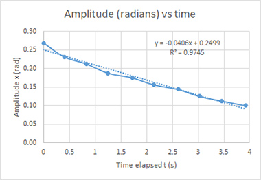 |
| Graph 1 shows the decreasing amplitude of the ball as it rolls back and forth. The period T is 0.98 seconds. | Graph 2. The amplitude in radians plotted against time. The slope is -0.040 rad/s. |
The gradient was -0.040 radians/second. Using Rod Cross's formula I obtained a co-efficient of rolling friction of μ of 0.0070. The next thing to do would be to try different diameter balls - but I have exam papers to mark.
Air Cannon
Projectiles such as tennis balls, oranges and
potatoes can be launched from a plastic pipe using compressed air. The device is
called an air cannon and relies on a cylinder of air compressed with a bicycle
pump being quickly released into a smaller plastic barrel via a quick-acting
valve (hand operated or solenoid). There are many designs on the internet but
for the purposes of a good EEI a small cannon should be made and the pressure
restricted to a maximum gauge pressure of about 30 psi (200 kPa) for safety. You
could examine the effect of pressure, barrel length and diameter on distance.
Most of the designs on the internet look dangerous and may be classified as a
Category B Muzzle Loading firearm under the
Queensland Weapons Act (1990) because it could do "bodily harm" (bruising) so negotiate the design and safety considerations
with your teacher (see "weapons"
note above). If in doubt - don't do it.

Another air cannon
The photos below show the design of a typical
air cannon. The rule here is simple, if you can't carry this out safely
after having done a risk assessment, including arranging appropriate adult
supervision, and meeting any legal requirements - don't even think about it. In
fact, in Queensland, a compressed air gun like this is a classified as a
Category B Muzzle Loading firearm under the
Queensland Weapons Act (1990) because it could do "bodily harm" (bruising) so negotiate the design and safety considerations
with your teacher (see "weapons"
note above). If in doubt - don't do it. It could be that it can only be
used by a person with a Category A/B firearms license, either on a range or in a
rural area with a property owner's permission.
To anyone considering it, check
before a breach of the Act is committed. It would seem very dangerous
though - a small fracture in the pipe, a manufacturing flaw, or a weakened area
around the solvent adhesive, etc could result in sharp fragments travelling in
unpredictable directions. Under the Education Queensland guidelines it would
(probably) be classified as an "Extreme" risk activity that needed parent
consent and the Principal to sign off on the risk assessment.
 |
 |
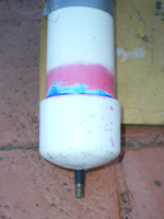 |
| The masterpiece. To see an enlarged view, click the image. | Pump up to 60 psi | Pump nozzle |
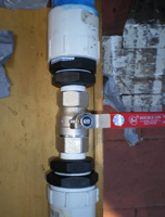 |
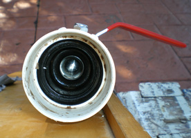 |
 |
| The expensive valve | The valve closed | The valve open and whoosh |
Air powered potato cannon
The other popular type of cannon based on the
above design is the potato cannon. The details are easy to find on the internet.
I was thinking that a good EEI would be to measure the range of a projectile
when the cannon is free to move (on wheels) or placed against a tree. Soldiers
know very well that if you place your cannon against the base of a tree you get
better range.
When a cannon is fired (restrained or free to move) the change in
momentum is zero, hence, mv0 cosθ - MV0 = 0. If the work done by the
expanding gases (W) is converted into the kinetic energy of the cannon (½MV02)
and the projectile (½mv02),
thus: ½mv02 + ½MV02 = W. Hence by combining the equations: ½mv02 + ½(mv0 cosθ)2/2M
= W. If the cannon is constrained the
formula becomes: ½mv02 + ½MV02 = W - U where U is the work done on the constraining tree. The rest of the
equations take too long to code for this webpage so you should have a look at
the linked article: Cannon recoil against tree.
I'd be looking at whether the recoil adds a certain % increase in range or
whether the elevation matters and so on. You should also see the "weapons"
note above.
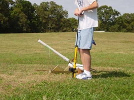 |
| Put the cannon on wheels and compare it to one staked to the ground. (Wellington Point State High School) |
"Windage" and air
cannons
To propel a projectile such as a cannon ball up a barrel it is essential
that the compressed air doing the pushing can't escape around the sides of the
ball. However, in the early days, because of irregularities in the size of
cannon balls and the difficulty of boring out gun barrels there was usually a
considerable gap between the ball and the bore - often as much as 5 mm - with a
consequent loss of efficiency. This gap was known as the "windage". The windage
of the guns was eventually standardised by trial-and-error: the bore diameter
was to be 21/20 of the gun's round shot diameter. As manufacturing precision
became greater it was reduced to 25/24.
On the SBS program "Engineering
Connections" Richard Hammond explained that windage was important in car engines
too. There should be a minimum gap between piston and cylinder. He fired two
projectiles out of an air cannon to show the effect of decreased windage (the
one with smaller windage
went 25% further in range). A good EEI would be to compare the effect of windage
on projectile range (keeping everything else constant). The projectiles would have to have the same mass but
perhaps you could make some wooden cylinders of slightly different diameters on the school's wood lathe
(but how would you keep the mass the same?). Over to
you.
 |
 |
| With the cannon ball placed in the barrel you can see the small gap. | Close-up of the windage (about 8 mm). |
Nerf Gun ballistics
You certainly don't need a weapons license for a Nerf Gun. They are
available at big toy shops like Big W and Target for a cheapish price. The Nerf
Gun fires foam projectiles up to about 11 metres. For an EEI you don't need lots
of power and range, you need something that has a convenient range to measure
accurately, and something in which variables can be controlled. There are many
Nerf Guns on the market - from about $12 to $49. There is no point in getting a
battery operated Nerf Maverick for $12.95 that shoots like a machine gun
(except if you're playing Humans vs Zombies on Halloween). Better to get
the Nerf-N-Strike Longshot Blaster for $49 which does a single shot from
a long (90 cm) barrel a distance of about 10 m.
You can vary the mass of the projectile by pushing weights into the foam, or you could alter the barrel length. Your main problem is how do you keep the pressure constant from trial to trial. Although a Nerf Gun could be considered a Muzzle Loading device under the Queensland Weapons Act it would not be considered a "firearm" as it could not do "bodily harm" (bruising). You should see the "weapons" note above.
 |
 |
The Nerf N-Strike Maverick is cheap ($12) but the
quick-firing is not much use in Physics unless Zombies are on the loose. |
A much better option for a Physics EEI is the Nerf
N-Strike Longshot CS-6 for about $45. Also a great present for your
Physics teacher. |
Sliding off a roof
Particularly in colder climates, the problem of
objects sliding off a roof is a big problem - mainly snow and ice - and many
steps are taken to ensure this happens in a controlled way. A similar situation
arises in amusement parks - particularly water slides - where the designers need
to calculate the landing position of a person for a given incline angle,
friction, and height of the launch point above the ground. For the diagram below
the relationship is: mgL sinθ
- μ mgL cosθ
= ½mv2. From
this you can calculate launch velocity and hence horizontal range on landing.
You could do a great EEI by considering these factors and seeing how they relate
to your experimental data. What angle gives the greatest range - and why; and is
this for all coefficients of friction? You could also consider a rolling object
but rotational kinetic energy would also have to be considered.
 |
 |
 |
| Observations to be made | An EEI that is going to end in tragedy. | Stanthorpe State High School perhaps. |
Measuring projectile velocity acoustically
In the two experiments above, the range of the projectile is considered to be a
measure of the velocity of the projectile. A neat EEI would be to compare
methods of velocity estimation rather than just the factors that influence the
range. I have seen an interesting method in The Physics Teacher (Nov
2007, Volume 45, (8), pp. 496) in which a microphone hooked up to LoggerPro or
some other data recorder is used to measure the time elapsed from the initial
explosion to the time taken for the sound to return from the target. You need a
big metallic target like a thick sheet of aluminium placed say 10 metres away.
Once the projectile strikes the target the sound is returned to the microphone at the barrel (muzzle) of the cannon. You get a waveform like the one below. The first part is saturated by the gas pressure as the projectile rushes up the barrel and the second point is when the sound returns to the microphone from the target. If you can work out the speed of sound you can subtract the time for the sound to return from the time after the ball leaves the cannon. v = s/t and you have your answer. Is this more reliable than a measure of range? How does range method and the acoustic method compare? Which is less prone to errors? Could you try 20 m rather than 10m? The possibilities are endless.
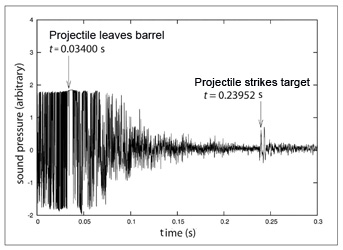
Parachute descent and mass.
Parachutes are not only used for sport but for dropping soldiers into war zones
and delivering food and medicine to flood and drought ravaged countries. Even
though they've been around for several hundred years it wasn't until after WW2
that the apex vent was invented. You could do an EEI to find out how drop time
is affected by mass, canopy area, size of apex vent, number or length of
strings, canopy shape and so on. That's Genevieve Ash on the right having a bit
too much fun. Click here to download
Moreton Bay College's Year 10 Parachute EEI task.
 |
 |
| Parachute terms | Genevieve Ash doing her EEI at Moreton Bay College way back. |
Arrow range and draw
A bow is a device that converts slow and steady human force over a distance
(Work) into stored Elastic Potential Energy (in the form of tension in the Bowstave, Limbs, or Prod). This energy is converted into Kinetic Energy upon
release of the Bowstring, and a great deal of that kinetic energy is transferred
to the arrow. A bow is basically a spring which stores energy to be put into the
arrow. However, 'draw' is not necessarily proportional to the force applied; and
therein lies the complication. You could examine range vs. draw for an
interesting EEI.
You could consider a comparison of velocity by
ballistic pendulum and by the range formula. A bow and arrow is not considered a
"weapon" under the Queensland Weapons Act (even though it could be lethal - but
so could a baseball bat or kitchen knife). It only becomes a "weapon" when used
for a "behavioural offence" such as attacking a person. You should see the "weapons"
note above. Some good advice on archery safety procedures is given in the Archery Australia Policy Number 1018 "Safety Guidelines" (2011) on their Policy and Procedures Website.
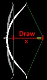 |
 |
Arrow elevation and range
When you fire an arrow from a bow you will see that different angles of
elevation give different ranges. In a vacuum it can be seen that the maximum
range occurs for an elevation of 45º. However, in air, the range and elevation
are not related so simply (see the two graphs below). This suggests several good
EEIs. You could merely find out which elevation gives the best range when "draw"
is kept constant, but you could also propose an hypothesis along the lines of
"45° gives the greatest range" and that angles above or below this give a
shorter range. Further, complementary angles are said to give the same range -
but this could be tested (see diagram below). Lastly - is "range" the only
dependent variable you want to look at. Perhaps an archer is more interested in
"time of flight" as this may give better accuracy (less time for air resistance
to apply). I have attached two pages from my New Century Senior Physics text
that may be helpful in designing this experiment. Click here to download them.
For safety information about archery, see the comments in the EEI suggestion
above.
 |
 |
||
| Theoretical path of a projectile (in a vacuum). Complementary angles seem to give the same range - but is this true in practice? | In air the path is somewhat different. This is for a cannon shell going to great heights - not an arrow. | A protractor stuck to the bow and with a brass bob hanging down is one way of measuring the elevation angle. | Practice firing by Year 11 Physics students at Wellington Point SHS, Queensland. |
Arrow accuracy and tail fletches
Tail fletches are the feathers on the ends of arrows. You could do an accuracy
comparison of Bulldog, Native and Pope & Young fletches; or you could try
setting the fletches straight with no offset, straight with an offset, or left
and right helical fletching. The combinations are enormous. You could
investigate the errors with different fletches; why? What's the hypothesis?
What is important - range or accuracy & why?
For safety information about archery, see the comments in the EEI "Arrow Range
and Draw" suggestion above.
 |
 |
 |
| Three common methods of trimming feathers. | Remember - the string on a Recurve Bow goes on the outside of the curve. Students often get this wrong. | One way to measure long ranges. But how accurate is it? |
Slingshot range and draw
You could always make your own slingshot and test
out how it goes for different angles and amount of draw (pull-back). One student
(Jack) at Kuranda State High School (North Queensland) made a huge slingshot
using steel waterpipe and 8 mm thick speargun rubber. He worked out the spring
constant in the classroom and then looked at conservation of mechanical energy
in his big slingshot on the oval. He varied angle, draw and mass of projectile as his independent variables; and range was the
dependent variable. The photos below
came from his EEI. My thanks to his Physics teacher Ruth Moxon for getting
Jack's permission to use these photos. Note:
Slingshots are not "firearms" at present under the
Queensland Weapons Act 1990 but there is a concern that commercial slingshots
can be lethal. Of particular concern to police is the Saunders Falcon 2 Wrist
Rocket Slingshot type which can be quite lethal. It may be described as a
weapon in changes to the Act (you should check;
and you should see the "weapons"
note above). The one
shown in these photos is not likely to be of any concern under the Act.
 |
 |
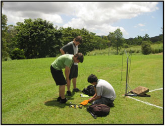 |
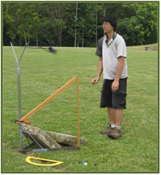 |
| The frame | Measuring the spring constant | Getting ready to fire | The launch |
Measuring "g" using falling nuts
Most attempts to measure the acceleration due to gravity end in disappointment as the errors in timing or from friction are
a big problem. This suggestion requires the use of a set of steel nuts tied
together with string at set intervals, and a microphone and CRO. Basically, you
hold the nuts-on-a-string vertically and drop them on to an aluminium pie plate.
The impact sounds are captured as a series of peaks on the CRO which allows you
to measure the time intervals. The diagram below shows the setup. If you don't
have a CRO in the lab, download a free sound analyser (Audacity or Scope for example). Click here to see my
note about computer CROs further down the page.
As it stands you have an experiment that could be done in the lab in a double lesson. Is this good enough for an EEI? No, you'll need to extend it so that you are using an hypothesis of some sort to guide your development of a procedure that extends the idea of measuring g with falling nuts. You could investigate ways to improve the accuracy of the method, you could look at the relationship between the measurement of g and other variables (weight of nut, spacing of nuts and so on). To get an "A" requires a carefully thought out plan of manipulating variables and detailed examination of all the uncertainties and errors you've coped with. Good luck. Get plenty of photos.
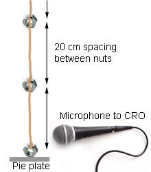
Measuring "g" using a bouncing ball
A neat way to measure 'g' experimentally is by using a bouncing ball (eg a superball). As it bounces the sound of each successive collision with a hard surface can be captured using a microphone and a sound recording program such as Audacity. From that you can work out the time interval between bounces. The key to the experiment is that the height of each successive bounce is a constant fraction of the previous height. This constant fraction is called 'restitution' and could be in the order of 0.7 for a superball on a hard surface.
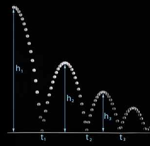 |
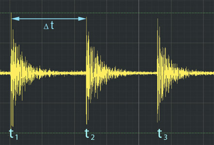 |
The ratio of h2/h1 is a constant (k) called the 'restitution'. It should also be equal to h3/h2. |
The time between the first and second bounce (t2 - t1) can be read off the CRO screen. At half-way in between the ball would be at the top of its flight. |
I got this idea from the work of Oliver Schwarz, Patrik Vogt, and Jochen Kuhn - Physics educators from Germany. The free-fall time of the ball from its maximum height h2 (where it has zero velocity) until its impact is half of the time Δt between two impacts (t2 - t1). By using this and knowing that restitution (k) = h2/h1, and using the distance-time law for free fall, g can be obtained. I won't show you here as that is for you to work out - but it is only Year 11 kinematics.
How do you make an EEI out of this? You would not be just trying to measure the value of 'g' at this location. You would need to investigate the conditions under which this result is the most reliable. You would vary the starting height (h1) and see if that affects accuracy, and if their is some relationship between accuracy and the conditions of the experiment. You are bound to get different values for 'g' for successive bounces - but why is that? Do they vary in any sort of systematic way, or are they random.
Rise of bubbles in soft-drink, champagne and beer.
When you open a bottle of soft drink you get a hiss of gas escaping around the lid but you also get fizz of bubbles in the liquid itself. If the drink is warm, the formation of bubbles can be rather explosive. This is hardly new to you but the physics might be. Because gas solubility in drinks increases with pressure, the sudden reduction of pressure when a bottle of soft drink (or champagne or beer) is opened causes the gas to exsolve, forming bubbles. But if you look at the bubbles rising you may notice that they double in size by the time they get to the top. They also appear to accelerate upwards. See photo below (by Gerard Liger-Belair, taken from "Effervescence in a glass of champagne: A bubble story" in Europhysics News).
 Shafer and Zare (1991) took high-resolution and high-speed pictures, found that bubble growth rate is roughly constant. The pursuit of bubble physics is more than pure academic curiosity and pleasure. And it makes a good EEI. See their paper here.
What causes a bubble to rise? The answer of course is that the density of a CO2 bubble is less than the density of the surrounding liquid. The buoyancy force Fh is proportional to the volume of the liquid displaced by the spherical bubble (Archimedes' principle):
Vbubble x (ρbeer - ρbubble) x g = Vbubble x ρbeer x g.
(Assuming the density of the bubble of air is inconsequential compared to the density of the liquid. Note: Vbubble can be replaced by the volume formula 4/3πr3, and thus the buoyancy force is proportional to r3.
As a bubble rises, it encounters a frictional drag force that is a function of its radius and speed as well as of the viscosity, density and surface tension of the liquid it is in. If the ascending bubble had a fixed size, it would reach a constant velocity when the (upward) buoyancy force exactly counterbalanced the (downward) drag force. However, the bubble's radius is always increasing due to extra gas coming out of solution and into the bubble (and not due to decreasing hydrostatic pressure as is commonly thought). Thus the drag force, which increases less rapidly than r3, can never quite catch up to the buoyancy force, which is proportional to r3. In other words, the upward buoyancy force increases more quickly than the downward drag force, causing the bubble to accelerate upwards.
This explains why in a stream of bubbles rising from a nucleation site on the beer glass, the bubbles near the bottom are smaller, slower and more closely spaced than those near the top. For example, a bubble with a radius of 0.5 mm rises in beer at 90 mm/s, but a bubble with a radius of 0.03 mm rises at only 1.0 mm/s.
Although bubble radius varies linearly with time, bubble speed increases with time. This suggests a great EEI. My thanks to Brisbane Physics teacher Mike Hennessy who's students have completed many successful EEIs on this topic (and thanks, he says, to the parents who were willing to open lots of champagne for their sons and daughters to video bubble rising in slow motion). To collect data, all you really need is a thin ruler of some sort that can be placed in the bottle of drink when it is opened, or glass of drink when it is poured. Of course, a camera with high speed capabilities would be good. The iPhone6 works well for instance. The rest is up to you.
Speed of sound in air as a function of temperature
For his Year 11 EEI Chamara Perera from Wynnum
State High School (Brisbane) made use of the coldroom at MacDonalds where he
worked after school. Here's what he said:
"The pictures (below) show the length of PVC pipe placed on a piece of ceramic tile (to ensure a crisp echo), with the microphone placed at the opening of the (closed) pipe. I found that the click of a pen worked really well when used to make the noise to echo, registered very clearly on the computer. The older version of the program 'Audacity' was used as the recording program, I say older program because that one measured down to more significant figures whereas the new doesn't. Measurement was then taken from the peak of the first registered noise to the peak of the second. To vary temperature, I took this very apparatus to the fridge at work which was about 5°C, the freezer at work, -21°C, outside on a cold night, about 11°C, up into my roof on a hot day about 30°C and finally just at room temperature, about 24°C. All temperatures were measured vary accurately using a temperature probe and the program Logger Pro 3.4.5".
As a matter of interest Chamara obtained a
resonant frequency of 240Hz at 4.2°C,
246.8 Hz at 21.1°C and
248.3 Hz at 25.8°C (I won't
include all his data as you have to do this for yourself). The
questions you could ask are: did you try other lengths of pipe; was the
frequency of the sound important; did you try other independent variables; what
was the source of any errors; is there a phase change upon reflection and is
this a problem, what are the limitations of the experiment; why is this
important to you and to society...and so on.
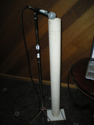 |
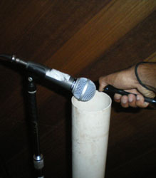 |
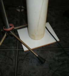 |
| Full setup | Making the click | The reflecting end |
Resonant frequency of an
open pipe - when "open" is not so open.
A fascinating EEI can be made out of a pipe experiment similar to the one
above - but using an "open" pipe. If you slap one end of an open pipe with a
piece of soft foam (rubber 'thong' or 'flip-flop', or even a piece of
polystyrene foam) the air in the pipe resonates. The loudest frequency is the
fundamental providing you have chosen a pipe of suitable length that resonates
in the audible range. A length of 60 cm is a good start. When the compression
wave travelling down the pipe meets the outside air at the end, the wave is
partially reflected (and partially transmitted). It is the reflected wave that
sets up the resonance condition that you will have learnt about in class (f =
v/2L). You need to include end correction into your calculations ( = 0.6133r
for each end).
However,
here's the question: what constitutes an "open" end? If a ceramic tile (or any
hard surface) was placed 1 cm away would the end still be "open"? What if it
was 10 cm away - and so on? I tried this and found a delightful result.
Yes, from about 0.75 cm to 6 cm there is a variation in resonant frequency but
outside of that - nothing. The experiment is quite simply done but - be warned
- the physics of gas behaviour at the end has not been studied much and would
challenge university physics students. But this doesn't mean you can't get
some great data to explore; and discuss the situation in high school physics
terms. This would be a fabulous EEI.
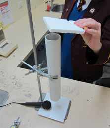 |
 |
| Here's the setup I used at Moreton Bay College to trial this. The hand belongs to Jade - who was slapping the end of a plastic pipe with some polystyrene foam. The microphone was connected to a computer running Soundcard Scope (but any similar program eg Audacity would work). | Here's the graph of our results. I have purposely left the scale off the x-axis so that you can't just use these results. The distance from the tile to the open end of the pipe varied from about 0.75 cm up to 7 cm. The temperature, length of pipe and internal diameter must be recorded. |
Hydrogen explosions - the origin of the 'pop' sound.
At some stage in science class you will have tested for hydrogen gas by placing a lit match to a test tube full of the gas. You would have heard the distinctive 'pop' sound as it ignited. Wouldn't it be great if setting fire to hydrogen was your EEI?
Hydrogen is likely to be the most important future energy source with the potential to make significant reductions in greenhouse gas emissions. Safe use of hydrogen by the public requires that the safety issues have to be investigated. Its behaviour in accident scenarios has to be predicted, allowing safety measures to be developed where necessary. A key factor in this process is predicting the release, dispersion and combustion of hydrogen in appropriate scenarios. Investigating the events of a hydrogen 'pop' in a tube can be most instructive.
A hydrogen 'pop' by students Morgan and Erin at Our Lady's College, Annerley, Brisbane.
When a test tube of hydrogen gas pops, a flame front travels down the tube as the gas burns. The temperature rises quickly to 3000K. Because it is so explosive, a compression wave (with a pressure of about 7 atmospheres and speed of some 3000 m/s) travels down the tube and possibly reflects off the closed end and then travels back up the tube in the heated gaseous products. In the video you can see where I recorded the 'pop' with the audio program Audacity. From that you can analyse the waveform for frequency and see if it varies with time. Does the frequency or 'envelope shape' depend on the diameter or length of the tube (for Physics students); or even the H2/O2 ratio (for Chemistry students). This is so much fun. I've analysed the sound from the clip above using Soundbooth and Audacity and it looks like the images below. If you want a audio recording of the pop to try out, click here.
 |
 |
Programs such as Audacity or Soundbooth (above) can be used to analyse the sound. The big peak comes 0.023 s after the sound starts and it has a frequency of 1000Hz. |
Audacity Spectrum plot of the sound from the video. |
Plasma Speakers - "Can't touch this"
Often a student will ask if a "plasma speaker" would form the basis of a
good EEI. Plasma speakers are a form of loudspeaker which varies air pressure
via a high-energy electrical plasma instead of a solid (cone) diaphragm as in a
normal speaker. When the plasma speakers are connected to the output of an audio
amplifier, the plasma glow discharge acts as a massless radiating element,
creating the compression waves in air that you hear as sound. In essence it is a
circuit that produces a high frequency voltage modulated by an audio frequency
(some variants simply use the 555 Timer IC for this). The modulated result is
fed to a flyback transformer (via a power Mosfet) to produce a high voltage high
frequency arc. The audio modulation of the arc causes it to produce (Low-Fi)
sound. However, the high voltages and heat involved make this a real
electrocution and fire hazard. Physics teacher Craig Airton from Tannum Sands
SHS (Queensland) said: "I had a student build one of these two years ago. It was fully
functional and had quite impressive sound quality, however, he burnt holes in the
carpet at his house and received electric shocks (not burns). I would not approve it again due to the high risk".
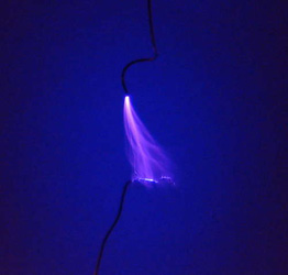 |
 |
| Plasma discharge (Indestructibles) | Home-made electrodes: a couple of nails in a piece of pine. Don't rest it on mum's carpet in the lounge room. |
If you are keen to see what they are all about have a look at The Indestructables - Plasma Webpage. What you must ask is "could it make a good EEI?" The
problem is, if you are doing a "manipulated variable" EEI then you have to
decide what variable you are going to change (the independent variable) and what
you are going to measure (the dependent variable). Then you have to propose a
hypothesis linking the two conceptually (and maybe mathematically) and then
provide a justification for your hypothesis using physics concepts, fact and
principles. No easy task for a Year 12 student. The chances of a good mark maybe
very slim so think carefully before you press ahead. In fact, when you do your risk assessment
you will probably find the hazards of electric shock, fire, UV radiation and
X-Rays are too great.
Guitar Pickup - 1
The electric guitar pickup works on electromagnetic induction principles. A permanent magnet induces magnetism in a steel string and when the string moves its magnetic field induces a tiny electric current in a coil of wire. This current is amplified after it leaves the guitar and fed into loudspeakers. The electric guitar pickup was developed in the 1950s and has changed little over the following 60 years probably because it was so simple and worked so well. It makes a terrific EEI.
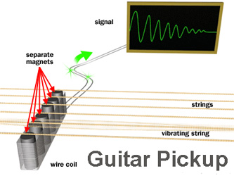 |
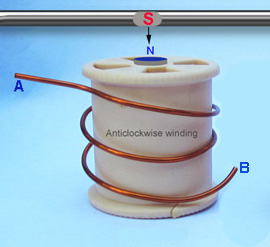 |
The six separate magnets are surrounded by a single coil of wire of about 5500 turns. The magnets are positioned directly under each string. On many guitars the magnets can be seen to be different distances away for different strings, and the arrangement has to be suitable compromise for picking up vibrations of the thick "bass" strings and the thin "treble" strings. |
A mock-up of a single pickup coil to show the direction of an anticlockwise winding (as viewed from above). When the south pole in the string (shown in grey at the top) moves towards the coil a south pole is induced at the top of the coil in accordance with Lenz's Law. The right-hand rule can be used to predict the direction of the current and which end will become positive (A or B). |
What variables can be used: the size of the current depends on the number of turns ("wraps") of wire in the coil, its resistance and the cross-sectional area of the coil. The most common arrangement in a real guitar is about 5000 turns of a very fine copper wire (42 gauge, 0.064 mm diameter, insulated with an enamelled coating (not plastic-coated that you are familiar with from the lab)). Varying the number of turns also varies the resistance. The induced current also depends on the magnetic field strength of the steel wire string, the distance between string and coil and so on. Lastly, the magnetism in the string depends on the strength of the permanent magnet, its distance away, and the size of the string.
You can see there are many variables to explore. What you may have trouble with is investigating how well the vibrating frequency of the string is reproduced by the coils. Because the current in the coils is alternating you will get a capacitance and inductance effect that is dependent on the frequency. The coil described about seems to have an optimum frequency of 7.4 kHz so you may need to work out how to tension your string to get this sort of value as a starting point. You may also need to work out where to place the pickup along the string and where the string should be plucked (plucked midway may give the fundamental but guitar players tend to play the strings about 1/7 of the way along to get rich overtones - but do you want that complication for a Physics EEI?).
 |
|
I used an electric drill to wind the coil. I just put a bolt through the spool and inserted it into the chuck of the drill. You can get 0.25mm diameter enamelled copper armature from Jaycar for $7 for 65 metres. |
Girls at Moreton Bay College used a digital tachometer that we bought from Jaycar (Cat. QM1448) fro $80. It worked flawlessly. Just put some reflective tape (supplied) on the chuck of the drill and point the laser in the tacho at it and away they went. Perfect. |
Rules of thumb they use are: the more windings you put on, the stronger the signal output, but higher frequencies will suffer; thinner wire cuts high frequencies more than thicker; tall skinny coils give a cleaner sound and shorter fat coils sound more "dirty". Guitar players often wind their own pickups (Eddie van Halen for example on the homemade Frankenstein Stratocaster-style guitar used for his classic Eruption).
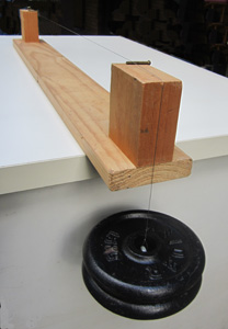 |
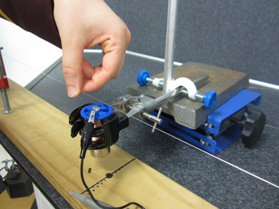 |
I made up a sonometer with a piece of pine 85 cm long with wood at either end to raise the string. Strings are about 110 cm long. |
The coil has a steel bolt through the middle with a rare-earth "super" magnet underneath. The lab jack is used to raise the coil to the right height. My thanks to Georgina for the photo. Her group (with Georgia and Shannon) wound various coils from 200 to 800 turns. |
Some hints: Guitar strings come in various diameters but you need to get "plain" ones that are not wrapped with additional wire. The wrapping they use is mostly nickel or stainless steel which complicates the design of the experiment. The first 3 strings on a guitar (high E, B, G - that is the highest pitch ones (closest to the ground) - are plain. The uppermost 3 (D, A, low E) are wound. I chose the G-string as it was the thickest (0.016 inch - commonly said to be "16 thou" referring to it's diameter of 16 thousandths of an inch. They never refer to diameters in metric (0.4064 mm) even in a metric country like Australia). The string has a "ball end" which is a little brass cylinder that you can fit a screw through. Make sure you get plain steel though, and not a iron-nickel alloy string.
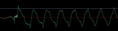 |
 |
You could use a CRO to analyse the output but I thought I'd try a computer's sound card. I connected the two wires from the coil to a 3.5mm mini jack and plugged it into the microphone socket (pink) on the computer. I captured the waveform using Adobe Soundbooth (with the gain turned right up as I had just 300 turns on the coil). The frequency measured was 75.6 Hz. |
Using Audacity I also got 75.6 Hz. I found that picking the string with a stiff-bristle artist's brush kept the interference to a minimum. With effort you could get a cleaner waveform. Good luck. This promises to be a fabulous EEI. If you can't get a signal check that the microphone is selected as the input device in the audio mixer. It can be very frustrating if you don't get the input selected properly. |
Where to get the rare-earth magnets? If your school doesn't have a supply, you can buy them or pull them out of old hard disk drives. Secondly, manufacturers and hobbyists dip their spools in melted wax for about 20 minutes to get rid of air bubbles. Should you? This gives them more consistent results (as well as lowering their resonant frequencies a tiny bit); so 'yes', if you have time, do it but it is not critical for an EEI. What about the wire? The finest enamelled copper wire is 42 gauge which sells (as 'magnet wire') on eBay for $7 for a 2000 m spool; Jaycar (Australia) doesn't have wire this fine - but they have 33 gauge wire - 0.25 mm diameter - 60 m for $7. A coil of 600 turns on a cotton reel with takes about 60 m of the 0.25mm enamelled wire. Ideally you would use finer wire and more turns - perhaps 5000 to 8000 like they do on real guitars.
Guitar Pickup 2 - The Humbucker
A simple guitar pickup with one coil ("bobbin") of wrapped wire (as described above) is called a single coil pickup. Look at any original Stratocaster built between 1954 and 1979, and you will see three single coil pickups (below).
 |
The Fender Stratocaster showing the three sets of single-coil pickups. In 1977, the middle pickup was changed to "opposition" by reversing the direction of the wire wrap and changing the polarity of the magnet. When pickups 1 and 2, or 2 and 3 were used together the hum was cancelled but the strong signal from the string was retained. This was equivalent to the Gibson Humbucker. |
Single coil pickups are good in one way but bad in another. The good way is that they produce a "twangy" tone that many guitarists like. The single coil tone is a sound that has become closely identified with the Stratocaster. The bad news is that single coil pickups are subject to outside signal interference, resulting in "hum" or "noise" because the single coil will pick up a variety of stray fields from nearby equipment.
Gibson guitars, by way of comparison, employ a dual coil pickup, which are essentially two bobbins wired in opposite directions that "cancel", or in Gibson terminology, "buck" the single coil signal interference: the classic "humbucker". Stray magnetic fields passing through the loops induce opposing currents and the result is zero current. Hence - no hum.
However the magnets in the two coils are also reversed: in the first coil of the humbucker, the magnets are North pole up; in the second coil, the South pole is up. That makes the induced currents add, giving more output and a "fatter" tone.
 |
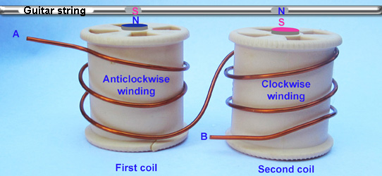 |
Gibson Humbucker. The two bobbins (each with six magnets) are connected "in opposition". The idea of reversing one loop of a pair to minimize interference has been around since its invention by Alexander Graham Bell in 1881. Telephone wires were twisted together ("twisted pair") for this purpose. More recently, the principle of common mode rejection in audio recording relies on this idea. |
A mock-up of the two coils of a Humbucker. Imagine a stray magnetic field ("Hum") threading the loops of both coils in the same direction (say increasing downward). The coils would oppose this change by generating fields in the upwards direction with and "A" would become negative. For the 2nd coil "B" would become negative. The two currents would oppose each other and cancel out. However for a string moving towards the coils the currents would add together to produce a strong signal. If you are discussing this in your EEI you'll need to refer to Lenz's Law and explain the process (I'm not going to tell you). |
So it has social and economic importance. So, how to make an EEI out of this? You could investigate how effectively the humbucker cancels noise from different directions (over, under, sideways, down) while still doubling the wanted signal. I'd be looking at the Common Mode Rejection Ratio (CMRR, measured in decibels) as a function of your manipulated variable - whatever you choose it to be. This EEI would require a considerable amount of research to design a worthwhile investigation.
Guitar Pickup 3 - Different loads on a guitar pickup
To follow on from the EEI suggestions above: one thing that guitar hobbyists argue about is the effect of different loads on the pickup? The three basic elements of passive electrical circuits interact in the guitar pickups, cables, and load, and all affect the signal that finally reaches your ears. These three elements are resistance, inductance, and capacitance. The general term impedance is used for all three or any combination of them. One this they discuss is the value of boutique cables (see below) - special low resistance, inductance or capacitance cables that are said to give a sweeter sound or other such vague claims.
 |
According to the U.S. manufacturer of Zerocap cables:
|
The output from a pickup is an alternating current and as such responds differently to the type of cable it is being fed through. You could investigate the effect of capacitive loading by comparing the output of a pickup with a normal length cable, an outrageously long cable (maybe a 50 m roll with connectors attached to each end) and a normal cable with a test box that puts different capacitors and resistors in parallel with the pickup. You could also look at the effect of frequency because capacitive impedance drops as frequency increases, and inductive impedance rises - so there is a trade-off. Here's a comment from a guitar hobbyist's blog:
When you play with "hot" (low impedence) pickups for the first time, their sensitivity and output level are impressive. There's plenty of signal - sometimes enough to overdrive even what you don't want overdriven. If you want to blast an amp into distortion this is the way to go, punching out every last watt with every pluck or strum. But play soft, or turn your guitar down for a clean sound, and you may be disappointed. Where are those soaring highs, the clean brilliance, the crisp bite you got with your original pickups? Why do chords now sound so dull? Suddenly your hot pickups are only lukewarm. Could it be the cables? People say that long cables can dull your sound. But why only with these pickups? What's going on here? Keep your cables as short as possible! Half the length means only half the capacitance. If you must run long ones, use high quality, low capacitance cables. [Website URL - http://www.howardmickdavis.com/LoadingandCables.htm] |
This is not an EEI for the faint-hearted. It is complex and has complex physics principles behind it. You would only attempt this if it all makes sense and you can see where you are heading. Be warned - without adequate theory to back up your design and discussion it may be nothing more than a hobbyist's "trial-and-error" Saturday afternoon project and unworthy of an "A".
Factors affecting the
frequency of an organ pipe
This is another music-related investigation you could undertake - but it
also applies to the exhausts of motor cars and bikes; for example, auto
engineers make the exhaust pipes such that they resonate at certain desirable
frequencies. For some V8s with a separate tailpipe from each bank of
cylinders they run a 60mm pipe down each side and put a 50mm pipe joining them
to generate beautiful beats. So organ pipe physics is used all over the place!
Why not investigate end correction for different wavelengths and diameters of a
simple pipe (eg PVC plumbing pipe); and for open and closed pipes. How does
temperature play a part?
 |
 |
 |
|---|
Spacing between successive turns of a slinky suspended vertically under its own weight
Here's a good one if you like playing with toys. When suspended vertically,
a slinky will stretch enormously even under its own weight, its extension being
tens of times greater than its undistorted length L0 when not hung,
depending on the size and material of the toy. Here are two suggestions: Suggestion 1. Suspend the slinky from any turn along its length and let
the rest of the n turns below it dangle freely. Then measure the free-hanging
length as a function of the number of turns in it, L(n). Physicists have
calculated that L(n) = (mg/2κ) n2 where κ and m are the force
constant and mass of a single turn, respectively. See reference below. Suggestion 2: choose a slinky such that when suspended from the
ceiling freely it stretches nearly all the way to the floor (a longer one may be
cut to size). Measure the distance from the bottom end as a function of the number of
turns, y(n), as you advance up from the bottom of the slinky (L0 is
the full length of the stretched spring; L = length of the spring unstretched
(lying on it's side), y = distance from bottom up to turn n; N = total
number of turns. Physicists have derived a formula for this:
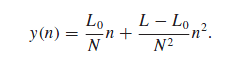
For either: What is the effect of added mass; why would anyone want to know this - what's the point? Compare a steel and plastic slinky. How do their spring constants vary? Source: Paul Gluck (2010). A project on soft springs and the slinky: Physics Education V45(2), p 180.
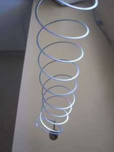 |
 |
|---|
Magnetic Field in a Slinky
The availability of inexpensive Hall Effect
magnetic field probes enables an interesting EEI to be done into the magnetic
field strength inside a slinky. You can insert the probe beteen adjacent turns
(see photo below) and measure the field as a function of the distance between
turns (or turns/metre). For a second variable you could try changing the current
or placing the probe at different distances from the centre. However, if you
don't have a Hall Effect probe (eg from Vernier Software) and want to make your own there is a good article
(for download) in Physics Education V45(5), September 2010, page 529.
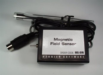
Hertzian Waves
Many early experiments with radio used sparks as detectors and as sources of
electromagnetic radiation. A good EEI would be to investigate the
electromagnetic nature of radio waves. You could find out if the strength of the
signal decreases of intensity with distance from the transmitter, and to
investigate electromagnetic shielding. One way would be to tune a transistor
radio (not digital) between stations. The radio almost certainly has an
automatic gain control and so will be more sensitive when tuned between
stations. However the background noise - also broadband noise - will be stronger
too. Hold one end of the wire to one end of a 1.5V battery. With the other end
of the wire briefly scrape the surface of the other battery terminal, making
sparks that will be visible in dim light. You could use a CRO to measure the
loudness of the crackle on the radio. What happens with distance, voltage of the
transmitter, shielding (paper, metal, glass) between transmitter and receiver.
Speed of Sound in a Metal Rod (see four
approaches below).
An experiment commonly used in first year physics at university is to determine
the speed of sound in a metal rod. If you use metal rod clamped at the centre,
standing waves can be formed in the rod by striking one end of the bar (end on)
with a hammer. Since the bar is clamped at its mid-point a node forms there
while antinodes form at the free ends as shown in the diagram. If the bar is
vibrating in its fundamental mode, then the wavelength of the wave in the metal
is equal to twice the length of the bar (L). So fair = f rod;
hence vrod = frod× λ = frod ×
2L. You'll get a lot of (odd, 3rd, 5th, 7th ...) harmonics thrown in but
the fundamental should be the strongest. So what variables are you going to
manipulate to make a great EEI. Some continuous variables are: Perhaps see if the velocity is constant for different lengths. Does temperature affect the speed? Some
discrete variables to manipulate are: What about other nodal
positions: can you suspend the rod to get the 2nd harmonic and how does the
speed compare when it is vibrating in the 1st harmonic? What about other metals; what characteristic of metals (Young's
Modulus perhaps) provides a continuous variable that can be tested. The error
analysis for any of these will be so important.
The following gives you some ideas about some techniques that may work well:
Speed of Sound in a Metal Rod 1 - Microphones and CRO.
The frequency of the standing waves in the rod is equal to the frequency of the sound produced and this can be determined by using a microphone connected to a CRO, or if you have it, DataLogger Pro or similar. You'll get a lot of harmonics thrown in but the fundamental should be the strongest. So fair = f rod; hence vrod = frod× λ = frod× 2L. You may be lucky enough to have access to a computer program that analyses the sound from the microphone (may have to amplify) and applies a Fast Fourier Transform technique (FFT) to convert the frequencies being received to a spectrum of amplitude vs. frequency: the largest peak amplitude being the fundamental frequency of the rod or bar. One student struck a problem with this method: she used a 20 cm rod of steel of 0.75 cm diameter and got a frequency of 2500 Hz using LoggerPro. This corresponds to a speed of sound in metal of 1000 m s-1 instead of 5000 m s-1 as expected. There's a great article in Physics Education about this (see caption below).
 |
 |
| This diagram has been taken from a great article in Physics Education 35(6) November 2000 entitled "Measurement of the speed of sound in a metal rod" by Se-yuen Mak, Yee-kong Ng and Kam-wah Wu from The Chinese University of Hong Kong, Shatin, NT, Hong Kong is attached for research purposes only (click link to download). If you have problems getting a trace on your CRO see the note below. |
Paige Kurmass from
Thuringowa State High School, Queensland, gives the thumbs up as
everything is working in her EEI. She used apparatus as shown in the
diagram to the left with different lengths of steel "reo-bar" and
determined the effect of temperature on the speed of sound. In her
Conclusion in the EEI she commented on the problem of reflection of
sound waves from the walls of the lab, and problems in heating such long
lengths of rod. |
Speed of Sound in a Metal Rod 2 - Electromagnetic method
Another good method is to use an iron or steel rod with a loose coil wrapped around one end. If the rod is slightly magnetized (as it is in the Earth's magnetic field), the increased density at the compression maximum will be accompanied by an enhanced magnetization. When this region of higher magnetic field passes through a pickup coil placed around the rod (see Fig. 1), an EMF will be induced. The signal, consisting of a series of pulses, may be fed directly into an oscilloscope. This method is described in The Physics Teacher V40, Jan 2002, p56-57 (attached for research purposes only - click to download). If you have problems getting a trace on your CRO see the note below.
 |
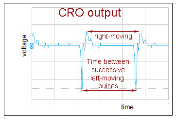 |
Speed of Sound in a Metal Rod 3 - Time of Flight method
If you use a setup as in the diagram below and strike the end of the rod with a hammer, the CRO will record the initial hammer strike (Channel 2), then the sound at the far end that has travelled through the rod (steel, about 5000 m s-1 for a longitudinal wave and about 600 m s-1 for a transverse wave) on Channel 1, then lastly the sound of the hammer blow that has travelled through the air (340 m s-1) again on Channel 1. If you have problems getting a trace on your CRO see the note below.
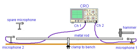 |
| Hitting the rod
laterally (on the side) as in this diagram will favour transverse waves
(v = 600 m s-1 in steel). If you want to get longitudinal
waves ( v = 5000 m-1) then you should hit the rod on it's
end. |
Speed of Sound in a Metal Rod 4 - Transverse Resonance.
The setup used in any of the suggestions above can be used to general transverse waves. To do that you have to hit the rod on the side near one end - at right angles to the rod. It will then vibrate like a tuning fork prong. The node will still be in the middle and you'll still get the first harmonic where λ = 2L. However, the speed of sound due to translational waves is about 1/8 of the longitudinal speed. There is a formula to work out the speed: v = √(2πfcK) where c = √(Y/ρ) and Y is Young's Modulus for the metal (200 x 109 N m2 for steel), and ρ is density (7800 kg m-3 for steel) and K = radius/2. So for a steel rod 5 mm in diameter and 20 cm long: v = 630 m s-1 for a transverse wave. This is about one-eighth of the value for the longitudinal wave.
Note about digital CROs. If you are after cheapish computer-based CROs you can get a "Focussz" Chinese 44MHzUSB-CRO on ebay for about $40. I bought one (it works well but I have problems with adjusting the display, and the manufacturer www.focussz.com won't reply. There is also a less-useful 5 kHz one for $25 from a different company and may be okay for most EEI uses. However, there is also a free (to schools) software one called "Soundcard Scope" that uses the computer's line-in socket on the audio card. I have downloaded it and tried it out and it is quite remarkable. I struck a 440Hz tuning fork at the correct position for a pure tone and the software gave me 440.3 Hz. Not bad for a free CRO. It is written by Christian Zeitniz from Germany and is available at http://www.zeitnitz.de/Christian/scope_e. If you have problems getting a trace on your (non-digital) CRO see the note below.
 |
 |
Soundcard
Scope by Christian Zeitnitz - in voltage mode |
Frequency
analyser mode |
I bought a bunch of 20mm diameter aluminium rods of varying lengths(1.8m down to 30 cm)from the local metal dealer (he cut the ends perfectly square as you need for "singing rod" experiments). I held them vertically at the middle (to cancel transversewaves) and struck them square on the end with a steel hammer and they "sang" beautifully. Using the microphone, I collected the signal on the CRO. It was a bit messy as it had many overtones present but when I used the "frequency analysis" option it showed the big fundamental and all of the overtones as a histogram. You could see the various overtones die away in real time. I did this for all of the rods and the calculated speed of sound in the rods was almost all identical. I plottedf (y-axis) vs 1/(2L) and the gradient is the velocity. I got 5035.76 m/s whereas the accepted value is 5091.8 m/s. There are many great EEI possibilities in this setup. PS: I bought my 20mm aluminium rod from Brisbane Steel Supplies at Capalaba for $33.20 for a 4m length (cut to size for free). One hint passed on to me by a teacher who had problems getting a signal (it kept switching off): some computers have an echo cancellation option that is automatically switched "on" and has to be checked "off".
 |
| Here's a screen capture showing the fundamental
frequency of a 1.200 m singing rod and a frequency of 2104 Hz. Click here to see a larger version
plus some notes. |
Another note about CROs
This is NOT an EEI suggestion but a couple of helpful hints from Alan Whyborn of Urangan State High School. If you can't get a trace on your CRO from a microphone you could:
1. Check the range switch on the probe: most probes have a range switch on them to switch between 10x, 1x and sometimes earth (to get a zero baseline). Make sure the probe is NOT on the earth position. (The input channel controls also have an AC/DC/ground selector - make sure you don’t have it switched to ground).
2. Channel selector: ensure you have selected to display the channel to which the probe is connected.
3. Triggering: this is quite likely to cause the problem (if the trigger level is set beyond the range of the input signal you won’t get a trace on some trigger settings). Make sure the trigger is set to the input to which the probe is connected and adjust the trigger level until you get a trace - or try setting trigger to auto.
4. With the signal generator, if it is one of the earthed mains powered generators you MUST make sure you have the polarity on the connecting wires correct. Otherwise you will simply short out the output via earth and get zero signal reading. If it is a battery powered (hand held) generator it shouldn’t be a problem - these are generally "floating" and have no earth. (worth noting here that the earthed mains powered signal generators only need ONE wire, not two, to complete the circuit, so if you have an RCA lead connected to the generator and a probe connected to the CRO you only need to connect the probe to the centre post and ignore the earth alligator clip. This MIGHT introduce a bit of 50Hz interference but compared to the generator output it should be negligible)
5. Most mics will only produce a very small voltage unless they are powered (perhaps a battery in the mic) so you will have to set the range selector on the input to a low voltage setting.
6. Make sure the vertical offset is not adjusted so high (or low) that the trace is off the screen.
7. If none of these work, maybe you have a short in the wires you are using. If the CRO is measuring DC voltages it SHOULD work fine for AC, so I would doubt it is a fault with the CRO (unless perhaps the fault is in the trigger circuitry, but that is not likely).
Good luck. Alan Whyborn - Urangan State High School
Speed of sound - resonance method
One of the important investigations carried out
by professional scientists is to improve the accuracy of physical quantities
such as specific heats, resistivity and so on. The National Physical
Laboratory in London was set up in the early 1900s to do just that. As
part of the investigation they look for errors in methods and try to minimize
them. This idea can form the basis of many EEIs - that is to extend simple
experiments by extending the range over which variables are measured or to
improve accuracy in existing methods. One simple but excellent experiment is
carried out in high school physics labs throughout the world: the measurement
of the speed of sound by resonance, in which a tuning fork is held at the end
of a close (at one end) tube and the tub's length varied until resonance
(loudness) is heard (see photos below). The length of the tube can be varied
by immersing it in water. A good EEI would be to measure the speed of sound
using the first harmonic condition (pictured below) but trying it for a range
of frequencies. Is there a relationship between frequency and the speed? If
there is we have a problem that bears investigating.
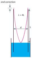 |
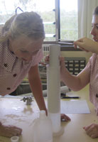 |
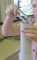 |
| Moreton Bay girls seek
resonance |
||
Speed of sound - is "end correction" really that
correct?
Following on from the description above - just
how correct is the end correction formula: e = 0.4d ? The end
correction is the amount of length you have to add to the value for the length
of the air column to get a correct value for the speed of sound. It is like a
"fudge" factor but can be justified by physics theory.
 |
My thanks to Brianna for letting me photograph her during the experiment. Where was everyone else in her group? Good question. Taking photos of themseves in slow motion I think. |
It would be interesting to see how accurate this factor is. For the first harmonic λ = 4(L + 0.4d); for the next harmonic, the third harmonic (remember only odd harmonics with a closed pipe) λ = 4/3 (L + 0.4d). If v = f λ and v and f are constant then the velocity for the 1st and 3rd harmonics should be equal. You can solve for "end correction". What of the 5th and 7th harmonics; and does it vary with temperature, diameter of pipe and so on. This would be a great EEI that you could do at home or in the bush. There are some terrific journal articles on this: I'd start with Pat Chiarawongse's IB paper on "The Effect of Diameter on the End Correction of an Open-Ended Tube".
Speed of Sound - using the
stereo microphone input of a computer
The little "ear bud" headphones can be used as microphones if they are
plugged into the microphone socket of a computer (pink socket). They are poor
microphones but are good enough for a physics experiment to measure the speed of
sound. If the left and right earbuds are placed 1 metre apart then a sound
coming from one side, in line with the earbuds, will take about 0.003 s to get
from one to the other (t = s/v = 1.00/330 =0.003 s, assuming that sound travels
at 330 m/s in this example). If you use audio capture and analysis such as Audacity or Adobe Soundbooth you can measure the time fairly accurately. If the earbuds are far
apart you get a more accurate time but the intensity of the sound at more
distant earbud is reduced and hard to analyse. It is a tradeoff between time and
intensity. I tried earbuds 10.5 cm apart and made a sharp noise by hitting a two
steel bars together. I found that by hitting a glass bottle with a steel rod I
got a sharper sound.
Some earbud types don't seem to work. The white ones that
come with an i-phone or Mac work really well. The waveform is shown below. The time seems to be
0.000305 s which gives a speed of 344 m/s. The air temperature was
20°C. This
seems to be spot on as the accepted value for sound at
20°C is also 344 m/s. There's a good article on this
in The Physics Teacher V50, May 2012 p308 where Patrik Vogt and Jochen
Kuhn from the Department of Physics, University of Kaiserslautern, Germany,
discuss further investigations. They try putting the earbuds in plastic bags and
measure the speed of sound in a trough of water. A good EEI would to be try
different distances and measure the times. Theoretically, a graph of t vs d
should go through 0,0 and if it doesn't this may give you clues to a systematic
error in the measurement device. I tried it and got a perfectly straight line
going through 0,0 and the slope
gave a speed of 344 m/s, so 0% error; not too bad! Then you could try different gases, or
different temperatures, or water, or tape them to a steel rod, a wooden bench and so on.
 |
 |
| Screen shot of an Audacity waveform from my trial in which the earbuds were 11 cm apart. You need to remove all but the segment of the waveform that you want and then "amplify" it from the Effects menu. The red lines have been added to the image later. | Vogt and Kuhn obtained a time difference of 1.49 ms with their setup, having the earbuds 50 cm apart. They calculated the speed of sound in air to be 336 m/s. accepted value is 344 m/s at 20°C. |
Time dependence of static friction
This is going to be a tricky one and I haven't seen it done in a high school lab before. The research question posed is: how does static friction vary with contact time? That is, if you leave a block of wood sitting on a bench, is static (not dynamic) friction greater the longer you leave it. This is important in industry where detailed knowledge about static friction materials is required for the accurate calculation of the braking torque needed to hold a load at rest. This is particularly important for brakes in cranes, elevators, hoists and mining winding machines, which must meet specifications such as the definite value of the static safe braking factor. The study of static friction is also a useful supplement to the dynamic testing of brake friction materials.
The time-dependence of static friction can be explained by the fact that the real contact area is a function of time. The (weight) force on the surfaces in contact gives rise to plastic deformation and causes the material to creep. Perhaps you could get some similar objects (steel, aluminium or wooden blocks and leave them on a surface for different times and measure static friction). Perhaps an incline method would be more accurate (measure height rather than angle). I've attached an interesting article by S.F. Scieszka and A. Jankowski (Poland) from the Tribotest Journal V3(2) 1996 where they show that the coefficient friction is time dependent (by up to a maximum of 7-15%): ms = mo + c1t/(c2 + t), where c1 and c2 are constants. If you wanted to do it with low cost materials, I looked at using pine paddlepop (icypole) sticks and chopping one into bits and letting a piece slide down. Glued two bits together for a heavier object, then three. Hmmm, not happy! This could be a truly great EEI.

Rolling ball down an incline
I once watched my own children roll a ball down an
incline and as the incline angle was increased the ball sped up. However, there
came a point when it got slower even as the incline was made steeper. That made
me think it would would be a great EEI as it was a bit unexpected. Obviously
when the angle is 90°
it won't go far - but what happens at smaller angles. A good research question
is "for what angle will the horizontal speed be the fastest?" or if you are
measuring the time to travel across a table (see diagram below) "for what time
of travel across the tabletop be the least"?
An interesting discussion by Physicist Mark Lattery from the University of Wisconsin USA appeared in Physics Education (V35(2) March 2000, 130-131. (click to download). You really need to look at changing another variable to look for interrelationships in the data (size of ball, balls of differing restitution) as this is a key criterion for an "A" in IP3. This will be so much fun.
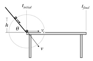
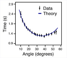
Bifilar pendulum
A bifilar suspension pendulum is one in which two
(bi) filaments (filar) support a rod. A schematic of this arrangement is shown
in the figure below. Bifilar pendulums have been used to record the irregular
rotation of the earth as well as to detect earthquakes. If a magnet is used
instead of the rod, the rate of oscillating can be used to measure magnetic
filed strength. If a plain metal bar is suspended symmetrically in the
horizontal plane by two strings of equal length and set to swing about a
vertical axis through its centre, the period of the swing (T) may depend upon
some, or all of the following quantities that define the system: the length of
the supporting strings L; the distance apart of the strings, s; the mass of the
suspended bar, m; and the length of the suspended bar, l.
There is a formula: T = KsmLn in which K is a constant and m and n are unknown indices. Thus: log T = log K + m log s + n log L. So if you do one experiment where L is kept constant and T measured for various values of s, then a graph of log T vs log s has a slope equal to m; and similarly, for another experiment you could measure T for various values of .... keeping ..... constant and then you could graph log T against log L and this will have a slope of .....! What a fabulous EEI.
Torsion pendulum
A torsion pendulum consists of a weight suspended
by a wire or some other fibre. The pendulum oscillates by repeatedly twisting
and untwisting about the axis through the centre of the wire. Though it is not
strictly a pendulum since it does not oscillate because of the force of gravity,
the mathematical formulas that describe the motion of a torsion pendulum are
similar to the equations that describe the simple harmonic motion of a simple
pendulum. It is commonly used in those ornate clocks in glass cases (see below).
For a bob of fixed moment of inertia and a wire of a given material, the period (T) depends only on the radius and length of the wire: T = KraLb where K is a constant, r = radius of the wire, L = length of the wire. Hence, log T = log K + a log r + b log L. Hence, if you use several identical wires (of the same type and radius) but different lengths, then a graph of log T vs log L should be a straight line of slope b. Also, if just the radius is changed then a graph of log T vs ......etc. Another great EEI in the making.
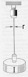
Cooking Meat I - Conductivity
Food technology is a massive industry and physics
principles can be applied to all facets. Physicist Dr Nathan Myhrvold worked
alongside astrophysicist Stephen Hawking before turning his attention to
cooking. He has recently released a 2438 page text on the science of cooking [Modernist
Cuisine, Ingram Publishers, 2011, $625).
He said most people thing that if a steak is twice as thick it should take
twice as long to cook it to the same degree. However, he says that this is
wrong and that heat conduction scales roughly as the square of the thickness
so it should take four times as long. This would make a fascinating EEI.
You would need pieces of similar meat but cut to different thicknesses. Different cuts of meat have different conductivity, with lean meat (low fat) having a higher thermal conductivity than fatty meat. The fibre direction also is important so there's a hint for a control. Government agencies define "cooked" as 70°C for 2 minutes (so does Mythbusters) so your best bet would be to see how long it takes for the temperature at the chosen positions (eg 1 cm and 2 cm) to rise to that value. It is also said that older animals have lots of connective tissue so "young" vs "old" may be interesting as another (discrete) variable. All you need is a lab hotplate and perhaps a few temperature probes and a datalogger.
Cooking Meat II - Conductivity and Different Heat Sources
The suggestion above describes the use of a hotplate as the heat source. A variation on that which would also make a good EEI would be to compare different heat sources. You could still use chunks of meat as above and still measure temperatures at say 1cm and 2 cm from the surface, and note how long it takes to get to say 70°C; but compare the hotplate with a microwave and convection oven. You'd need to have some sort of measure of the heat output of the various devices on the setting used - perhaps putting a known mass of water in a small beaker and heating that first (and use Q = mcΔT) and note the time taken to get a power (P = W/t) value. My thanks to Physics teacher and gastronome David Austin of North Bundaberg State High for his suggestion.
Cooking Meat III - Specific Heat
Similar to the
experiment mentioned above, you could also make a good EEI out of
investigating specific
heats of various types of meat. The specific heat will determine how fast a
piece of meat cooks. Lean meat is said to be the lowest specific heat at about 0.85 kJ/kg/K
whereas fatty meat is about 0.95 kJ/kg/K. Bone is much lower at about 0.60
kJ/kg/K but this depends on how dense the bone is. You may need to develop a
method based on ones you may have used for measuring the specific heat of
brass, or look at the procedures used in food technology laboratories. I would
look at heating a chunk to say 100°C in a laboratory oven and then dropping it
in to chilled water (why chilled?).
The problem you'll have is developing an hypothesis and justifying it. It is not much good for an EEI just to measure specific heats and leave it at that. You should be trying to extend knowledge about factors that affect meat specific heats and why it may be important. Talk to your teacher and look at the criteria sheet in detail before you get too carried away. I'd be thinking there is some relationship with moisture content or fat content. You could weigh a chunk of meat and dry it out for many hours in an oven, and then reweigh it to get % moisture. To measure % fat, you could extract the fat with hexane or some other non-polar solvent, and then evaporate the solvent. Plenty of methods are on the internet.
Hot Air Balloons
Physics teacher at Urangan State High School, Hervey Bay, Queensland - Alan
Whyborn - has his students investigate hot air balloons and the conditions
needed for the balloons to catch fire. He said that he once saw a
colleague in Canberra make hot air balloons from shopping bags, using
metho and cotton wool, simply wired across the handles of the bag. They took
them outside (on a still day), lit the metho and off they flew. On a number of
the bags the opening collapsed in a little and the bags caught alight. He was
horrified at the sight of flaming balloons releasing drips of burning plastic as
they drifted casually through the air! He says: "In August 2007 in Canada, a fire broke out in
a hot air balloon. Two people were killed. Could it be that the air in such a
balloon may become excessively hot and cause the material of the balloon (the
"envelope") to ignite and burn?" This sounds like the basis for an EEI:
factors influencing the ascent of a hot air balloon.
Alan gives the following important tips: large,
really thin/light garbage bags must be used, and get the lightest cane available
(craft shop). Also, if the balloons are allowed to fly to the ceiling, they can
tilt and the bag might catch fire, so the anchor is very important (plus it
holds the balloon in place while the pebbles are added to the gondola to
increase the payload). Also,
still air is necessary - inside the lab with fans off is great. If done
carefully with appropriate preparation and warnings, there is very little
hazard. In some cases, students have had a "fuel load" big enough to create
sufficient heat to shrink the bag. Ordinary cotton wool balls are perfect, but
not compressed or the rate of heat release might not be sufficient to get
necessary lift. Click here for: Procedures and safety
notes from Urangan SHS.
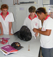 |
 |
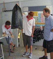 |
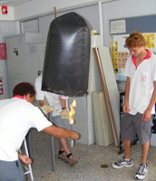 |
| Constructing: a light cane loop and sticky tape holds the bag end open. Fine wire across the middle is used to attach the fuel ball and gondola. | Fuelling: a cotton ball soaked in metho is attached by a hook to the centre wire. | Inflating: the ball is lit and the bag fills. A slack safety cord tethers the bag to the floor. | Loading: pebbles are added to the gondola to achieve neutral buoyancy. |
Slump of sandpile
You've no doubt seen reports on TV of kids
being buried on the beach when a sandhill collapses on them. The sand is stable
until someone digs away at the base. When bulk granular materials (like sand)
are poured onto a horizontal surface, a conical pile will form. The internal
angle between the surface of the pile and the horizontal surface is known as the angle of repose and is related to the density, surface area and shapes of
the particles, and the coefficient of friction of the material. Material with a
low angle of repose forms flatter piles than material with a high angle of
repose. The angle of repose, or more precisely the critical angle of repose is
the steepest angle of descent or dip of the slope relative to the horizontal
plane when material on the slope face is on the verge of sliding. Likewise, the
larvae of the antlions trap small insects such as ants by digging conical pits
in loose sand, such that the slope of the walls is effectively at the critical
angle of repose for the sand. When the ant walks on the sand it collapses and he
falls in to the hole. Now that's clever. A great EEI would be to measure the
angle of repose for different grain sizes of sand, or wet vs dry sand, or if it
is related to density and so on. Look up the triaxial shear test, or even
the direct shear test for ideas on how to measure repose.
 |
 |
| Angle of repose is
measured in degrees |
Antlion
sand trap |
Insulation and cooling of hot water
Bubble wrap is a good insulator but how would the rate of cooling of a
PET water bottle or a soft drink can of
hot water vary with the number of layers of wrap? Newton's Law of Cooling makes
reference to the rate of cooling and the difference in temperature between the
object and room temperature (but he also said 'in a gentle breeze' that most
Physics books forget to mention).
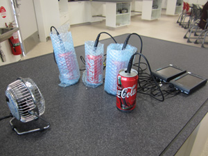 |
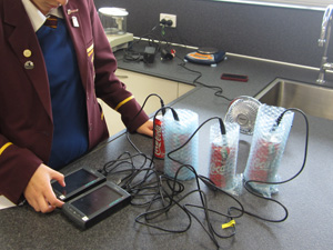 |
Year 12 Physics EEI at Moreton Bay College, Brisbane. Logger Pro makes life simpler. My thanks to Mackenzie for the photo (May 2015). |
Mackenzie has used a fan to simulate the 'light breeze' that Newton had when developing his law. See suggestion about 'cooling' and Newton's Law further down. |
Newton's law states that the rate of change of temperature is proportional to the difference in temperatures between the object (hot water, T) and the ambient temperature (Ta). Mathematically, this can be expressed as: dT/dt = -k (T - Ta). This is a differential equation and you can separate the variables and then integrate. This technique can be found on the internet. You end up with an equation: ln (T - Ta) = -kt + C. This takes the form y = mx + c, so a plot of ln(T - Ta) vs t (x-axis) should give a straight line. Here's an example from Mackenzie Petie:
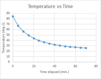 |
 |
| Temperature vs time graph for three layers of bubble wrap gives a typical exponential decay curve. My thanks to Mackenzie Petie for her data and graphs from her EEI. | Taking the natural log of the temperature difference gives a straight line whose slope (0.0146 minute-1) is the rate constant (k). This is also for three layers of wrap. The regression coefficient 0f 0.999 indicates that the data are a good fit for the line. |
Can you estimate what fraction of a layer of bubblewrap the polyester (PET) bottle or metal can is equivalent to?
Home Made Accelerometer
Accelerometers are devices for measuring the net acceleration force acting
on an object. In the computing world, IBM and Apple have recently started using
accelerometers in their laptops to protect hard drives from damage. If you
accidentally drop the laptop, the accelerometer detects the sudden freefall, and
switches the hard drive off so the heads don't crash on the platters. In a
similar fashion, high g accelerometers are the industry standard
way of detecting car crashes and deploying airbags at just the right time. Apple
uses an LIS302DL accelerometer in the iPhone, iPod Touch and the 4th & 5th
generation iPod Nano allowing the device to know when it is tilted on its side.
These are all pretty complicated but you could build a simple one from a narrow perspex or glass tank partly filed with a water and food colouring and mounted on top of a collision trolley. There is probably a relationship between the angle of the water surface and the amount of acceleration. I suspect you'll need a camera - maybe an SLR unless your compact has low shutter lag. Better still, mount your accelerometer on a spinning turntable and you'll be delighted for hours.
Photonics and fibre optics
The Australian Government's National Broadband Network is planned
to connect 90% of all Australian homes, schools and workplaces with broadband
services using fibre optic cable.
Understanding the physics behind fibre optic technology is set to become even
more important to those involved. As signals pass along the fibre they get
weaker (attenuate) as the light gets absorbed and scattered on its way through.
Attenuation is one of the most important measurements for optical transmission
systems because it determines the maximum distance between repeaters. With new
glass that has been developed for optical fibres, light can travel more than 10
km before 90 per cent of it is absorbed.
This is a big improvement over ordinary glass which loses 90% in 20 metres. Some interesting experiments involve modelling optic fibre with glass rod (eg stirring rod) and making different bends in a number of pieces. Compare energy losses ("curvature loss" or "macrobend loss") as a function of angle. Try dipping the rod in different liquids (to simulate the cladding) and measure the attenuation again. Try different thicknesses of rod. Put scratches on the glass. I'm tld that if the radius of the bend is greater than 20 times the diameter of the fibre, then losses are neglibible. Hmmm!
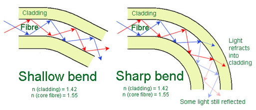
Bicycle Pump Thermodynamics
You are probably well aware that when you compress air quickly in a bicycle
pump the pump gets hot quickly. The energy imparted by your muscles is
transferred into heating the gas inside the pump and increasing the molecules'
internal energy. This is the same reason spacecraft get hot when they re-enter
the Earth's atmosphere - adiabatic compression (not friction). Diesel engines
rely on adiabatic heating during their compression stroke to elevate the
temperature sufficiently to ignite the fuel. If you had access to a temperature
probe and a datalogger you could mount the probe into a screw fitting and screw
it into the end of a pump. Let some masses compress the gas and take a few
readings. It's up to you what data to take and how to work out how much
mechanical energy is imparted to the gas by the falling masses. Is it okay to
assume that there is such little time for heat to escape to the surroundings
that Q (lost) = 0? Will the formula W = Fs be okay? Wikipedia has done a
lot of the hard work for you.
The Stud Finder
The stud finder is a device is designed to indicate the presence of wood studs
behind wallboard by detecting changes in capacitance. Generally, each detector
contains a capacitor whose conductive plates are arranged so that both plates
lie in the same vertical plane (see figure below). When the device is placed in
contact with a wall, that plane is parallel to the wall, causing electric fields
generated by the pair of plates to penetrate behind the wallboard. As the
detector is moved across the wall, those fields are affected by what dielectric
material is present, resulting ultimately in changes in capacitance. Those
variations are detected and then indicated by changes in light and/ or sound
intensities. For the stud sensor, the presence of a wood stud behind the
wallboard causes the capacitance to increase in that region due to an increase
in dielectric constant. For an EEI you could investigate the properties of a
commercial studfinder (about $25): do different wood types have different
capacitance; effect of moisture content of the stud; metal vs wood; electrical
cables (on and off); effect of thickness and so on. Perhaps you could make a
model one and compare. I should note that one student who did this had a lot of trouble getting useful results.

Magnetic Strength and
Distance
In World War 2, the Navy in Australia, Britain and the United States
received tens of thousands of suggestions about how to detect enemy submarines.
Most involved placing big magnets in the shipping channels. These were rejected
by scientists as being impractical because they knew magnetic strength falls off
alarmingly
with distance. However, it may not be a simple inverse square law ; it could be
inverse cubed. When you have the real world of dipoles
(N and S on the one object) the relationship is less clear. Here's what Wikipedia says about the relationship:
Far away from a magnet, the magnetic field created by that magnet is almost always described (to a good approximation) by a dipole field. One characteristic of a dipole field is that the strength of the field falls off inversely with the cube of the distance from the magnet's centre. Closer to the magnet, the magnetic field becomes more complicated and more dependent on the detailed shape and magnetization of the magnet. At close range, many different fields are possible. For example, for a long, skinny bar magnet with its north pole at one end and south pole at the other, the magnetic field near either end falls off inversely with the square of the distance from that pole.
So, for an EEI you
could investigate force vs distance for a pair of magnets. The diagram below may
give you some ideas. But is the "dipole" a problem. If you had really long
magnets then the second pole on each magnet may not be as important. That is, is
length of the magnet a variable?
 |
 |
Force between two
current-carrying wires.
If you've ever watched someone try to "jump start" a car with a flat battery
you may notice something funny happen to the wires. "Jumper leads" are two heavy
duty copper wires that are connected between the good battery on one car to the
flat battery on the second car. Positive is connected to positive, and negative
to negative. When current is drawn through them by the flat battery trying to
start, the leads move towards each other (if they are close enough). Ampere
devised a formula relating the length of the wires and the currents being
carried.
You could test this in an EEI but the formula may hold for an ideal case of very long (infinitely long?) wires. How does it hold as the wires are varied in length. That is, are there any "end effects"? And should the force be zero when they are at right angles (the textbook say "yes"). Here's a suggestion: use an electronic balance, hold a stiff wire (rod) in a clamp and blu-tac the other rod to the balance pan (see below). Solder (clip) lightweight flexible wires to the ends and connect to power supply (full-wave rectified?) and appropriate meters. Bob's your uncle.

Newton's Cradle and non-elastic collisions
Newton's cradle, named after Sir Isaac Newton, is a device that demonstrates
conservation of momentum and energy. It has no real-world application other than
as a toy. A typical Newton's cradle has a series of
identically sized metal balls suspended in a metal frame so that they are just
touching each other at rest. Each ball is attached to the frame by two wires of
equal length angled away from each other. This restricts the pendulums'
movements to the same plane. There are plenty of videos and demos on the
internet if you have not seen one live. They work well for steel balls; but what
about brass, what about lead. Is there a relationship between starting height
and final height when less elastic metals are used. It's no good just finding
out there is a difference without having some hypothesis to test. Is it a
density thing, or interatomic force thing? There must be some quantitative
difference between the metals that gives rise to observed differences in the
balls' behaviour. This will be hard.
Heating up gases
You would have seen how gases expand when they
are heated. Your teacher may have heated a flask with a balloon on the top to
show it expanding; you may have seen a balloon shrink when dipped in liquid
nitrogen at -198°C; and it is the principle behind how hot air balloons work.
In class you would have called the law describing the relationship between
temperature and volume Charles's Law or perhaps Amonton's Law (V
∝ T, when T is
in kelvin and P and n are kept constant). There could be a great EEI in
revisiting this relationship. There is no point in just verifying it as this
has been done a million times. What you want to do is to extend the
investigation of this law to look at the impact of changing variables and to
consider allowing for errors.
The diagram below shows a setup that may be useful. It really just show the connection of two things: a flask with a sidearm (maybe a Büchner flask) and a graduated glass syringe. The exact positioning is something you should determine. Glass syringes are precision-made with low friction between the plunger and the barrel (unlike plastic ones that have high friction). Your chem lab should have some and if not they are reasonably cheap (about $50 for a 100 mL one). You need to introduce a gas (eg CO2) into the flask and surround the flask with water in a beaker on a hotplate. As it slowly heats (I mean slowly, maybe 20ºC to 80°C over 40 minutes) the gas expands and the syringe is pushed out. With the syringe on it's side there is no need to worry about the weight of the plunger. You could compare gases - oxygen, nitrogen, hydrogen for example.
But how to get samples of these gases? You may have cylinders but you could produce H2 and CO2 by reaction (or let some dry ice sublimate); let some liquid nitrogen evaporate (or remove oxygen from air). And why not propane (BBQ gas) or butane (cigarette lighter fluid)? Remember that balloon gas is not just helium - it has 3% air mixed in with it. The main point is that the law holds for ideal gases but at atmospheric pressure and room temperature they won't be that ideal. And is the deviation from ideality dependent on the molar mass of the gas, or whether it is polar or non-polar, and where on earth do you get a polar gas from (HCl is too dangerous)? What range of temperatures will you use (consider liquid nitrogen, dry ice). What value will they give you for absolute zero when the V/T graph is extrapolated? How do you draw the line of best fit (is least-squares the best, does it give you the most accurate value for absolute zero?). And what is the volume of the gas in the apparatus? And what is the best way to measure temperature (of the gas as in the diagram, or of the water surrounding it)? Perhaps the temperature of the gas in the flask is the water temperature and the temperature of the gas in the syringe that of the surrounding air (work out a weighted average). And how do you control atmospheric pressure (do you have a barometer, or perhaps get the data from the meteorological bureau website). What a fabulous EEI. I must put this on the Chemistry EEI webpage as well.
The Heat Engine
You are probably quite familiar with things physicists and engineers
call "Heat Engines": the petrol and diesel engines for cars and trucks are
heat engines as they
convert heat energy to mechanical work by exploiting the temperature gradient
between a hot "source" and a cold "sink". The diagram below left shows this
process schematically. Heat is transferred from the source (Thot)
through the "working body"
of the engine, to the sink (Tcold) , and in this
process some of the heat is converted into work (W) by exploiting the
properties of a working substance (usually a gas or liquid). Even a "Dunking
Bird" is a heat engine (centre). This suggests a good EEI based on an
experiment often done in thermodynamics labs in 1st year university physics or
engineering. The diagram to the right shows the setup. It consists of a flask
connected to a glass syringe (see description in the "Heating up Gases"
suggestion above.
The heat engine works when the flask is shifted by hand from the cold water to the hot water and back again. The pressure of the system is monitored with the pressure sensor (to computer) and the volume of the system can be measured with the rotary motion sensor on the piston. You start with the flask in ice water and no mass on the piston. Then place a mass on the piston and the plunger falls. Then transfer the flask to the hot water and the piston rises. When it stops rising you remove the mass and then move the flask back to the cold water. That is one cycle. Some data I have from the American Journal of Physics (V 74 (2) Feb 2006, p 99) has Thot = 90°C, Tcold = 25°C, mass added to piston = 100 g, height lifted = 2.7 cm). With the right formula you get a value for Win (heat) = 29 mJ, and Wout (GPE) of 26 mJ giving a mechanical efficiency of 90%. Ask yourself - what is the source of energy loss? For an EEI you would need to research these formulas and the underlying theory and propose some variables to manipulate such as DT, mass, type of gas and so on. Whatever you choose you should have some way of justifying your hypothesis. Hard, but may be fun.
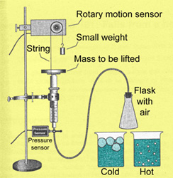
Datalogging Power Generation
The fundamental principles of electricity generation were discovered during
the early 1830s by the British scientist Michael Faraday. His basic method is
still used today: electricity is generated by the movement of a loop of wire
near a magnet (or vice versa). You could do an EEI on the factors influencing
the generation of an electric current. A good way would be to use a Pasco (or
similar) datalogger and record the voltage induced in a coil (air solenoid) by a
spinning magnet nearby (see photo). The experiment could be repeated with the
spinning magnet closer to the coil, or the number of turns on the coil can be
increased or decreased. These variations will cause the area for a half-cycle to
change, but again this can be shown to be independent of speed. If the number of
turns on the coil is changed by a known ratio, the area for a half-cycle should
change by the same ratio. You could also set up three coils at 120° to each
other. Photos courtesy of Mark Dixon, Clifton College, Bristol, UK.

The
Physics of the Bungee Jump
National Geographic magazine first reported this sort of jump by Pentacost Island natives
in 1955. It was later popularised by A. J. Hackett in NZ. The conversion from
GPE to EPE is an interesting one but the relationship is far from simple. You
could model a bungee using rubber bands and brass weights, or do something more
dramatic. You may even find out why they say bungee jumping is glue sniffing for
Yuppies. One of the problems is that as the jumper falls the mass of rope
hanging below is getting less so acceleration is actually greater than g.
That sounds wrong but it appears to be true. Have a look at: Understanding the Physics of Bungee Jumping from Physics Education V45(1) 63-72 (January 2010) and you'll see what I
mean.
What type of waterwheel is
the most efficient?
A water wheel is a machine for converting the energy of flowing or falling
water into more useful forms of power, a process otherwise known as hydropower.
In the Middle Ages, waterwheels were used as tools to power factories throughout
different counties. The alternatives were the windmill and human and animal
power. Overshot (and particularly backshot) wheels are said to be the most
efficient types; with claims that a breastshot steel wheel can be up to 60%
efficient (but who'd believe Wikipedia?). Why not make this the subject of an
EEI and see if efficiency depends on fall height, rate of flow, paddle area and
so on? Great fun if you're good at constructing things. But be warned - it's no
good just making a couple and testing them; you need to vary some of the
parameters and hypothesise how this may affect efficiency.
Flight of a Golf Ball
This was first investigated by Prof. Peter Tait of Edinburgh University in 1900.
His son was Scottish National Golf Champion who could hit a ball further than
the mechanics formulas of the time predicted because they didn't know about
spin. It still makes a great EEI as there are so many things to investigate.
Try: angle vs. number of dimples; try sanding off one-quarter of them and
putting gloss paint to make it smooth again; then try half (see below), and three-quarters. Design a device for giving it a constant velocity, eg falling pendulum, or
something spring-loaded. Vary angle, try at different speeds. How to get top
spin?

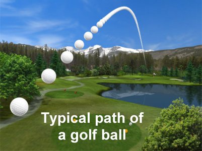
Gravity car
An old favourite for physics and engineering competitions is the 'gravity
car'. It involves the transfer of gravitational potential energy from a falling
weight to an attached small model car which acquires kinetic energy. There are
many designs but a simple one is shown below. The brass weights are attached to
a string passing over a pulley attached to the car. The string is wound around
the axle. As the weights fall and lose GPE, the string turns the wheels and the
car begins to move. Your EEI could investigate the optimum falling mass and cart
mass combination for maximum acceleration or velocity. Remember - as you
increase the falling mass (and thus DGPE) you are increasing the mass of the whole system. This will have
implications for acceleration. A great EEI and lots of scope for demonstrating
advanced thinking.
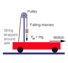 |
 |
 |
Components |
Alex Schumann-Gillett from Moreton Bay College used a Meccano "Buggy" car for her investigation. Alex is now doing her science PhD at ANU (2016). |
You can see the hanging brass mass that provides the driving force for Alex's car. |
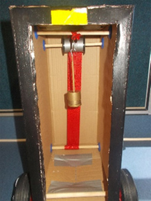 |
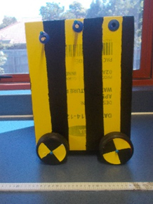 |
Inside the gravity car built by Codi Baker-Lahey - Year 12, St Andrew's Anglican College, Sunshine Coast, Queensland. |
Codi's car moving along the benchtop. |
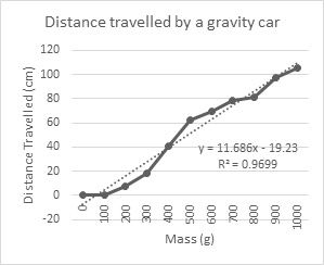 |
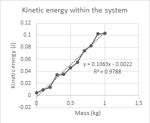 |
| Codi plotted total distance travelled vs hanging mass. | And here she worked out the kinetic energy of the car as a function of hanging mass. |
Descent of a ball bearing in oil or honey
It is vitally important that motor oil doesn't get too thin in summer nor too
thick (too viscous) in winter otherwise the car engine might seize. A Falling
Ball Viscometer uses the rate of descent of a ball bearing to measure the
viscosity of a liquid. Try investigating drop time vs. temperature, type of oil
(20W50 etc), size, mass or density of ball, width of column. This can be very
messy; oil is such a pain to clean up you're probably used to having someone
else clean up for you. So don't be surprised if your teacher seems reluctant and suggests you use honey. I wouldn't allow oil. The first thing you should read is about Stokes' Law and the variables within.
 |
 |
 |
A sophisticated setup using a Buchner flask to maintain a water jacket of constant temperature. |
Setup using honey - Villanova College, Brisbane. |
You can see the ball dropping through the honey. At 90°C it drops very fast (and how would you measure that?). |
 |
Viscosity of vegetable oil vs temperature - Moreton Bay College Year 12 EEI May 2015. Oil is such a pain because it is hard to clean up (well - for the lab staff to clean up). Harman is pouring hot oil into a big dish, and down the sink, and over the bench. |
Air
resistance and the descent of a balloon - #1 - Constant Velocity
Inflated party balloons fall slowly to the
ground because of their large cross-section for their weight (low density).
Students often think a good EEI would be to investigate the effect of air
resistance on falling objects (eg tennis, ping pong and cricket balls) but
mostly the objects fall too fast and the measurement error is too great. A great
EEI would be to suspend a motion sensor (ie a sonic ranger) from the ceiling and let
an inflated balloon fall from underneath it. You could increase the mass (add
paperclips etc) and redo the measurements keeping diameter constant. Then you
could keep the mass constant and change the .... (you work it out!). The main
things to look for are large lightweight objects such as
party balloons (recommended if you don't have a sonic ranger), plastic soccer balls, inflatable beach balls, styrofoam balls (eg the round
foam fishing floats in the photo below). Small weights can be taped on the
bottom or pushed into the foam; and you may need quite a large fall height.
The simplest experiment would be to look at the effect of these variables on terminal velocity. If you want to look at the accelerating phase as well then you should read the caution below. For terminal velocity you just need to work out when the balloon has stopped accelerating. Usually it is after about 1.5 m of freefall but you would need to establish that. Most students put two horizontal rods (eg rulers) about 1 metre apart vertically and time the balloon's descent between these two markers. If you put another marker 1 m under the bottom one and timed the balloon through the second distance, the time should be the same if it is at constant velocity. The downward force (weight) is balanced by two upward forces: buoyancy and air resistance. I'd be looking up Reynolds Number (no apostrophe) and Stokes' Law (with apostrophe). Remember that air resistance varies with velocity (squared). And that why this is a tricky (but
great) investigation for an EEI.
Air
resistance and the descent of a balloon - #2 - Accelerating
The simplest experiment is with constant velocity (above). A more complex EEI is to investigate the motion of a balloon while it is still accelerating (between 'let go' and terminal velocity). You need to be cautioned again that this is hard to do and difficult to analyse. When a large, light, spherical ball is dropped from a height (in air), it appears to descend slowly. It is obvious that the surrounding air has a profound effect on the motion of the ball, reducing its acceleration. One reason for the reduced acceleration is the buoyant force. This force acts opposite to the force of gravity and reduces the net force on the ball. There is also another effect of approximately equal importance. As the ball accelerates, it must also accelerate the air around it. Thus a ball moving through air has a larger effective inertia than one moving through vacuum. This increase in inertia also reduces the acceleration from the force of gravity acting on the ball.
The increase in inertia of an object moving through a fluid is usually called the "added mass". Even though this idea was discovered by d’Alembert in 1752, it is not well understood and is not dealt with in most introductory university physics texts. But the idea of added mass is used elsewhere in physics to account for oscillations of a massive spring or the motion of electrons in a crystal (where their effective mass is different from their mass in vacuum), and added mass is used to explain how neutrinos travelling through the Sun change their 'flavor' content, which is crucial for explaining the observed flux of solar neutrinos.
You can sum all of this up by using the familiar relationship: Net force = buoyancy force - drag force. However, net force is no longer ma (where m = mass of the sphere) as the mass is increased by the "added mass" (m'). So the net force is now (m + m')a where m' = mass of air in the balloon multiplied by a constant CM (which is approximately 1/2). There is a good article about it in American Journal of Physics, Vol. 79, No. 12, December 2011, p 1202.
Stability of a bicycle
Have you noticed how you can ride a bike with your hands off the handlebars and
you don't fall over? But if you give it a push just how long does it take to fall over?
Variables - linear speed, mass, angular
speed of wheel, rotational inertia of wheel I = mr2; add lumps of clay or lead to rim).
Sliding friction - variation with speed?
You've no doubt measured the coefficient of
friction by pulling a wooden block across various surfaces at constant speed and
measuring the force with a spring balance. Probably you've found that friction
is independent of surface area and normal reaction force (laws of da Vinci,
Amonton and Coulomb). That's fine but you might recall how
difficult it is to get constant speed. The problem is that friction does change
with speed (particularly for dry, unlubricated metals) although it may be not noticeable.
For steel, copper and lead, the frictional force seems to decrease with speed;
with Teflon it increases with speed; and in many cases complicated
relationships exist: for example, for steel sliding on polymers such as
polypropylene and butadiene acrylonitrile, a peak in the graph of friction
versus speed is observed. See Cross, R. (2005). Increase in Friction Force With Sliding Speed. Physics Department, 812-816.
A good EEI would be to have the setup shown below and then use trial and error (adding or subtracting masses from the hanging bucket) to get the block to slide at constant speed. Using a datalogger would do this fine. Then load up the sliding mass and add more masses to the bucket to get constant speed each time.
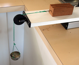 |
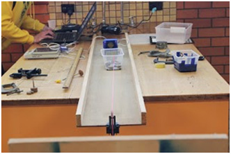 |
The hanging mass provides the force to pull the block along the horizontal surface. |
James Reich's setup at Villanova College, Coorparoo, Brisbane. The surface is painted Masonite (hardboard sheeting). James used a DataMate and plenty of trial and error. |
James Reich did this at Villanova College, Brisbane and found that the coefficient of kinetic friction does indeed increase as speed is increased. For example, for a constant velocity of 0.01 m/s the COKF was 0.693576 and for a velocity of 0.05 m/s the COKF was 0.694207.
 |
James Reich's tray of weights on the hardwood surface. |
Another good EEI would be to extend this
idea and measure the displacement or speed as a function of time as you add
different weights and try different surfaces. Think about grouping the surfaces
into elastically hard and elastically soft (rubber, textiles). Some computer interface packages
have a "smart" pulley that gathers data. The diagrams below may give you some
ideas. Perhaps a better way of measuring friction would be to measure the
acceleration of the system and using Newton's 2nd law (where Fnett is the calculated force accelerating the blocks and m is the total mass
of the system (both objects). The nett force will be less than the applied
force (the weight of the block) and the difference will be due to friction. A
good paper for background reading is "How to teach friction: Experiments and
models" by Besson, Borghi, Ambrosis and Mascheretti from the A.Volta
Department of Physics, University of Pavia, Italy in the American Journal
of Physics, December 2007, V 75, No. 12, pp 1106.
Pulling a nail out
Use a claw hammer to pull a nail out of wood. See suggestion below. Need to
compute mechanical advantage of lever. How
does force (calculate F1r1 = F2r2)
vary with depth of nail, diameter of nail, grain orientation (end, side, top),
density of wood. How does a pre-drilled hole (varying diameter) help or hinder? Scientific American had an article in about 2007. They said the force to
pull a 50mm nail out of end-grain of seasoned hardwood was about 260N, but the
force became lower as it came out. How would you measure the force as a function
of distance embedded. Now that's difficult!!
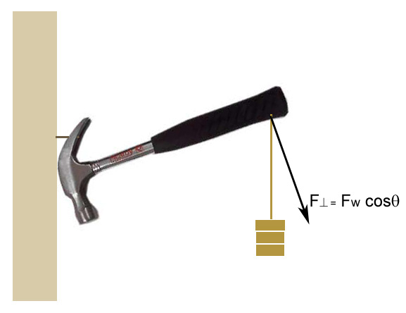
Cooling rates of water in a freezer
Some people say that warm water freezes before cool water but that seems to violate common sense and physics principles. This is known as the Mpemba effect, named after Tanzanian student Erasto Mpemba, who made this assertion in a paper published in 1969. Although there is anecdotal support for the effect, there is no agreement on exactly what the effect is and under what circumstances it occurs. At first sight, the behaviour seems contrary to thermodynamics. Many standard physical theory effects contribute to the phenomenon, although no single explanation is conclusive.
He pointed out that investigations of the phenomenon need to control a large number of initial parameters (including type and initial temperature of the water, dissolved gas and other impurities, and size, shape and material of the container, and temperature of the refrigerator) and need to settle on a particular method of establishing the time of freezing, all of which might affect the presence or absence of the Mpemba effect. The required vast multidimensional array of experiments might explain why the effect is not yet understood. There is a world-wide competition regarding these experiments. I'm told a Yr 12 student at Villanova College, Brisbane, submitted his Physics EEI and was placed 11th in the world.
If I were you I'd Google Mpemba Effect and take it from there. You could investigate some factors: Rate vs. container size, thickness or type of material, covered/uncovered, initial temperature, stirred/unstirred, temperature gradients from top to bottom of the container. Good one for thermometer probes and a computer interface, eg TI-CBL2, Casio, Datamate etc.
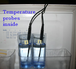
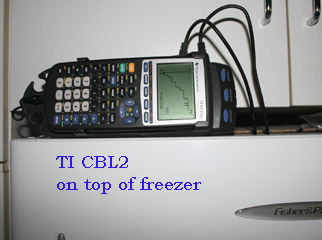
Elephants vs mice: surface area, volume and staying cool.
You may wonder how large mammals such as camels can survive in the hot climate of outback Australia - and maintain a constant body temperature while standing in the hot sun. The same is true of other big mammals - like elephants - in the tropics. The trick is that their surface area is small relative to their mass so that they can continue to absorb heat for the entire day without their temperatures rising to do any damage. Little mammals have a big surface area to body weight and are not as adept.
Here's a good little project that would make an interesting EEI. The aim is to study the surface area to volume ratio of an object. The area of a cube is 6L2 whereas the volume is L3. The ratio A/V is thus proportional to L2/L3 or L2/3. We can rearrange this such that A ∝ V2/3. If we can measure surface area as an object shrinks in volume we could verify this relationship. If we plotted log10A vs log10V we should get a slope of 2/3. That's the theory anyway.
 |
 |
Suspend the ice block on the hook under an electronic balance but wait until it starts to drip before you collect data. You can count the drips for a minute every 10 minutes or so. |
Here's a log/log graph of my results. I started with 120g of ice. The slope is not 2/3 like I expected but just 0.456. Not sure why but that's what an EEI is like. |
If we use a block of ice as the object we can measure its volume as it melts by measuring its mass and using the relationship m = ρV. The measurement of its surface area is more complex. A block of ice that is melting is getting its heat from the surrounding air. The heat that flows in is proportional to the surface area, and for every Joule that flows in a set amount of ice must melt (think latent heat of fusion of ice = 334 J/g). Thus the number of drops of melted ice that fall off the ice block per second is a measure of the surface area at that short moment in time. So we just need to keep a record of the mass and the rate of water droplets per second for various stages of melting and we have our data. If you want to collect data more simply just measure the mass as time passes and estimate the rate (drops/minute) frome the change in mass Δm. Too easy. One thing you must do it to wait until the block reaches 0°C and starts to melt. When it comes out of the freezer it might be at -10°C so you have to let it warm up to 0°C before it will start melting. Should only take 5-10 minutes.
In summary, the data are: (i) volume (proportional to mass), and (ii) surface area (proportional to rate of melting in drops per second). The premise is that as an object shrinks in volume its mass will shrink too but at a faster rate. See the suggestion below for some alternative ideas.
Iceberg Melting Rates
The melting and breaking up of polar ice has become an even more important issue since the impacts of climate change have been recognised. Research on the factors affecting the melting of icebergs has been going on for some time though; for example Dr W. F. Ross from the University of Melbourne was publishing his work in the Annals of Glaciaology back in 1978. In the EEI suggestion above I considered the importance for large mammals of the relationship between volume and mass (using a melting iceblock).
But this technique could be applied to an investigation of the factors affecting how fast an iceblock melts as it applies to climate change science.
It is well-known that the most important factor affecting iceberg melting is the temperature of the surrounding fluid (as you would have guessed). The fluid can be either the air around the exposed part of the iceberg or the warm water underneath (called 'basal' melting - which seems to be the cause of the ice-shelf loss in Antarctica). But other factors are the volume and shape of the icebergs. As stated in the suggestion above, the bigger the surface area (and in practice this also means volume) the faster the melting rate. When an iceberg melts it often cracks in two and, depending on the size and shape, has a 'rollover'. In the photo below you can see some different sized icebergs and these will have melted at different rates.
 |
 |
Can you predict which of these icebergs will melt faster? It is hard to tell their size but they are actually the size of office blocks. This photo was taken by Ted Scambos of the National Snow and Ice Data Centre during the 2006 IceTrek Expedition to Antarctica. Pieces smaller than 5 m are called "Bergy Bits" and pieces less than 2 m are known as "Growlers" (if they are also <1 m high). |
Block of ice with a drop just falling with a shutter speed of 1/1000s. I put the string in the water before freezing it. I also used boiled water to get a clear ice-cube. It probably should have been a uniform shape to start with - eg a cube. |
A good EEI would be to take an icecube and let it warm up and melt in the air. If it was attached to the underside of an electronic balance you could record its mass as time passed (see diagram in the suggestion above) - but only after it started to melt (see note above). The number of drops per minute would be a measure of its melting rate but so would be the change in mass per minute (much simpler). So work out its change in mass per minute (in g/min, or g/s, or kg/s - whatever you think best) and plot this against time elapsed (minutes, hours etc). A graph of mass vs time elapsed should be a curve; and the instantaneous slope at a particular time will be the rate. Plot that against time elapsed. This should remind you of some of the rate graphs from chemistry. This would be a fabulous EEI especially when you try to keep all other factors constant, and try to explain why two identical iceblocks melt at different rates.
Lastly, glacierologists often talk about the half-life (t½) of a melting iceberg. That is the time taken for its mass to halve (as in nuclear decay). The t½ for big icbergs (200 m wide) is about 0.5a, ie half an "annum" (year), whereas the t½ for 1600 m wide icebergs is 4a, but so many other factors come in to this. You could express your data like that (somehow). All yours.
Chladni Plate investigation.
You may have seen demonstrations of Chladni
Plates where a plate sprinkled with sand and attached to a vibrator is
caused to vibrate and a series of patterns emerges depending on the frequency
(see below).
It has societal applications: in recent years, there has been increasing interest in the positioning of micro-
and nano-particles on surfaces for the production of miniature biosensorsand molecular electronics. Chladni processes can be used to do this instead of
the slow and cumbersome lithography or prefabricated patterns
(e.g., by electrostatic positioning).
 |
 |
| John Daffron of Memphis USA was cutting out a circle in a large piece of thick aluminium with a dull band-saw blade, and the resulting vibration caused the chips to arrange themselves in a pattern of nodes and antinodes. He gave this photo to the Physics Teacher Journal where it appears in V50, Sept 2012, p 362. Looks like a ghost. Creepy! | Physics teacher Steve MacPherson at Wynnum State High School, Brisbane, demonstrating Chladni figures to a Year 10 Science class using a home-made setup. |
But even though they may be fun and look fascinating, as an EEI they
can be quite hopeless - so be warned!! Usually students increase the frequency
and note the value at which a stable patterns emerges and take a photo. This is
notnecessarily good EEI as there is nothing much to analyse; all you've
done is redo a demonstration that has been done a million times over the
past 220 years. However, you could also record the m and n values from
the pattern (by inspection; see middle photo below) and then analyse the results to see if Chladni's
Law is obeyed (f ~ (m + 2n)2 which it probably won't be but the
discussion can be all about the limitations. Perhaps comparing square
plates of different thickness (but same area) maybe more fruitful; or perhaps
square ones of same thickness but different areas. That way you'll be able to
manipulate two continuous variables (frequency and length). Student (Brianna)
from Wynnum State High made her Chladni plate vibrator from instructions at Instructables.
 |
 |
| A simple Chladni pattern on a circular plate. Here the student has generated one with n=3 nodal lines and m=0 nodal circles. | A "Sinai Billiards" pattern (complex, chaotic) generated by Yr 11 Physics student (Brianna) at Wynnum SHS during her EEI. |
Loop the Loop - measuring
"Jerk"
For an object travelling in a circle, its centripetal acceleration is given by ac=
v2/r. If it is moving in a vertical circle, its speed may change from
bottom to the top, so does its acceleration. The rate of change of acceleration
is known as "jerk" - units: ms-3. Examine the jerk of an object to model the motion of an
aircraft in a loop-the-loop. By the way - railway engineers try to keep jerk below 2 ms-3 to avoid passenger discomfort.
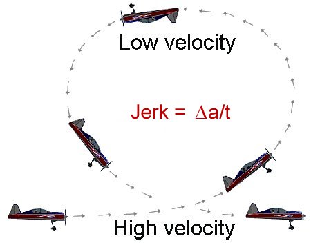
Effectiveness of sunscreens
To limit the amount of exposure to harmful UV
radiation, sunscreens are recommended. Suntan and sunblock lotions are two
different products. Sun blocks contain compounds like titanium dioxide or zinc
oxide that completely prevent all light from reaching the skin. Suntan lotions
contain compounds that absorb UV radiation and reduce the amount of UV radiation
that is absorbed by the skin.
The ability of a sunscreen to protect the user
from UV radiation is defined as the Sun Protection Factor (SPF). Some good EEIs
have been done on looking at the effectiveness of sunscreens in blocking
different wavelengths. It may be hard (and dangerous) to get a laboratory source
of UV so you could do it with just the Sun. I've seen some done with
light-sensitive paper to measure the sunlight getting through a thin film. Yr 12
Physics student at St Patrick's College, Mackay, Queensland, used different SFP
sunscreens smeared on Gladwrap.
Hot spots in a microwave oven
Your aim could be one of either (or both): to measure experimentally the
wavelength of microwaves in a microwave oven; and/or where are the hot spots and
how do they correspond to antinodes based on the answer to the first question.
Try investigating temperature rise vs. location; differences between horizontal
and vertical planes; which materials should I use - butter, chocolate, water,
grapes.
The photo on the right below shows a visualization of the horizontal mode in a microwave oven using infrared thermal imaging. A glass plate with a thin water film was placed at a height of 8 cm and heated for 15 s with a microwave power of 800Wwithout using the turntable. The antinodes are clearly visible. Source: Michael Vollmer (2004). Physics of the microwave oven. Physics Education, V39 (1), p 77.


Beam Deflections
Structures such as buildings and bridges consist of a number of components
such as beams, columns and foundations all of which act together to ensure that
the loadings that the structure carries is safely transmitted to the supporting
ground below. Normally, the horizontal beams can be made from steel, timber or
reinforced concrete and have a cross sectional shape that can be rectangular, T
or I shape. The design of such beams can be complex but is essentially intended
to ensure that the beam can safely carry the load it is intended to support.
Planning to do engineering at uni next year? Then why not get a head start and
do a "beam deflection" EEI?
Here's the scenario: as a structural engineer you are part of a team working on the design of a prestigious new hotel complex in a developing city in the Middle East. It has been decided that the building will be constructed using structural steelwork and, as the design engineer, you will carry out the complex calculations that will ensure that the architect's vision for this new development can be translated into a functional, economic and buildable structure.
As part of these calculations you must assess the maximum
deflections that will occur in the beams of the structure and ensure that they
are not excessive. It is said that the deflection of a spring beam depends on
its length, its cross-sectional shape, the material, where the deflecting force
is applied, how the beam is supported and so on. But perhaps this is only true
when you use homogenous, linearly elastic materials, and where the rotations of
a beam are small. I'm not going to give you too many ideas! Have a look at Scott
Boon's EEI photos below (Bundaberg North State High School, Queensland). He's an
engineer in the making. My thanks to teacher Mr David Austin for his help.
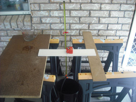 |
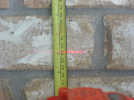 |
The load was water in
a bucket. |
Laser pointer helped
with accuracy. |
Settling velocity for soil aggregates
Water-borne soil erosion impacts on river,
estuary and marine resources and is therefore a major issue for Australian
agriculture and catchment management. It causes unsustainable losses of soil for
agriculture. Sediment eroded by water consists largely of soil aggregates (clay,
mud, fine sand, coarse sand, gravel). The settling velocity of such aggregates
and primary soil particles is of fundamental importance to the processes of
sediment transport and deposition in water. A great EEI would be to study
factors influencing settling velocity. A bottom withdrawal tube method is
commonly used for the direct measurement of the settling velocity distribution
of soil aggregates or particles of different sizes that settle together.
CSIRO and The Queensland Department of Natural Resources has been investigating the value of this technique for a range of soil aggregation and erosion applications. The simplest way is to take some soil - perhaps 5 grams - and add to a litre of water in a long plastic tube. Give it a shake and stand it upright and take off 100 mL or so every 10 s or so via a pinch valve in the bottom. Evaporate the water off each sample and weigh it. Methods are on the internet and are quite sophisticated. A fair bit of research will be needed to analyse and discuss your data.
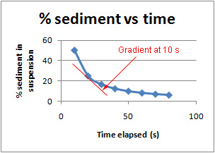

Hot ball bearing behaviour
If you place a hot steel ball bearing on parallel metal track
near a supermagnet, the ball sits there for a while and then zooms off. I have seen the video
clip made by Mr Mark Young and his former physics class at Churchie (some frames below)
but just what is going on here? Something to do with cooling below the Curie
Temperature. It
would be an interesting experiment to try. I have a hypothesis but have never
had time to test it.
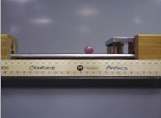 |
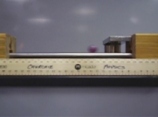 |
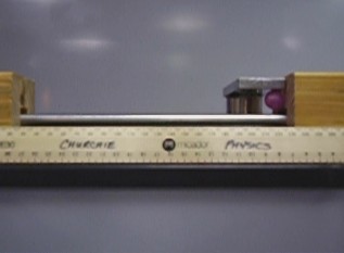 |
| Red hot - the ball bearing just sits there |
...and then takes off as it cools |
and smashes into the end at high speed. |
Carbon dioxide sound lens
Sound, like light, can be focussed using a concave reflector. Sound can also
be focussed using a refractor - just as a convex glass lens is used for light. A
biconvex gas lens will bend sound waves so that can be focussed providing the
gas in the lens has a density higher than the surroundings. You could make a
sound lens by filling a balloon with CO2 (from dry ice or a
cylinder). Your EEI could be to investigate
how the amount of refraction varies with the different densities of the gases
inside and outside the balloon, the degree of curvature, the relationship
between focal length and wavelength of sound, effect of temperature, ... the
factors are endless. If SO2 wasn't so dangerous you could try that
too.
There is an article, "A Balloon Lens", in the American Journal of Physics, V77 (3), March 2009 by Derek Thomas, Kent Gee and Steven Turley from the Department of Physics and Astronomy, Brigham Young University, Provo, Utah, USA. They inflated their balloon to a diameter of 60cm with CO2 gas and placed a loudspeaker 5m away. Their search region was on the other side of the balloon between 0 and 25 cm away from the surface, and about 14 cm either side of the centre line. They used frequencies between 3.18 kHz and 7.27 kHz. You could perhaps try a big piece of cardboard to act as a baffle around the balloon to stop diffraction around the edges.
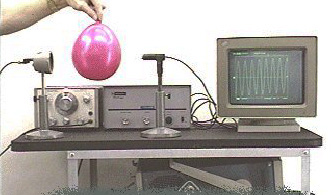 |
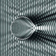 |
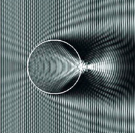 |
| Holding the balloon is okay for a demonstration but you would need to hold it firm. the loudspeaker on the left needs to be a fair distance away (eg 5 m) so that the sound waves reaching the balloon are essentially planar. | The scientists made a mathematical model of the sound waves going through a 60cm diameter balloon. This is the image for a frequency of 3636 Hz. | At a frequency of 7272 Hz the wavefronts are closer together and you can see the position of the focus more clearly. But does the frequency change the focal length. |
Submarine Buoyancy - "Up, up and away"
Submarines have been a source of wonder, awe, fear and excitement since
Bushnell built his Turtle in 1776. Super heroes and secret agents, in
both fact and fiction, have been in and out of them quite literally for
centuries. Scientists have gone to great lengths to show that the carefully
faked submarine adventure of Jack Sparrow in Pirates of the Caribbean was
physically impossible.
Here's a neat EEI from Sandgate State High School courtesy of physics teacher Ewan Toombes. It goes thus: Stage1 - Design and build a Robot Submarine using plastic bottle ranging from a 1.25L softdrink bottle up to a 4L juice container which can be trimmed to neutral buoyancy so that it "floats" just above the bottom of the pool at a depth of 1 metre. Stage 2 , The Escape - Release or inject a known volume of gas into the ballast tank(s) by remote control (something that operates above but works under water that allows you to inject a known volume of gas into your submarine) that will allow it to escape to the surface carrying a "treasure" of known mass that was resting on the bottom and attached to the submarine by a slack piece of string. Stage 3 - Measure the acceleration of the submarine as it rises. Stage 4 - Calculate the acceleration it should have had due to the excess gas and use your research to explain any difference between the two. That's the start. Now think of some variables to manipulate, propose an hypothesis, justify it, design an experiment and go and investigate. Photo taken at Sandgate SHS.

Slip or Tip - the limiting point for falling over
If you stand a wooden block on it's end and give it a slow push with a pointy
object (eg a pencil) it will either slide along or tip over. See figures below.
The question to investigate is: what factors influence the slip or tip height?
Is it friction, area of base, mass of block....? Amiee Leong (Year 12 Moreton
Bay College) gives it a go.
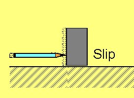
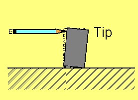

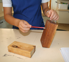
Coupled pendula
If you have a rigid horizontal support such as a rod between two retort stands
and hang two pendulums (pendula) of different lengths off the rod you get a
strange effect when you start one oscillating. The "rigid" rod is not quite as
rigid as you may think. It's not quite as simple as some books make out and in
fact makes a great EEI (particularly if you like a bit of maths). Using a
non-rigid support (called a Barton's pendulum) is much easier to get the
oscillations going.
Coupled pendula with springs
Another type of coupled pendula is shown below.
They are solid rods or strings attached to a rigid support much the same as the
figure above left (the broom). However, they have a lightweight spring attached
between them. There is a great article in Physics Education, Volume 45
No. 4, July 2010 about coupled pendula that provides background reading. Click
the link to download it. I have only provided some of it to avoid copyright
problems.

Battery discharge as a
function of temperature
You'd think that a frozen AA cell (battery) wouldn't work as well as one at room
temperature. But how true is this? The voltage appearing at the terminals at any
particular time, as with any cell, depends on the load current and the internal
impedance of the cell and this varies with, temperature, the state of charge and
with the age of the cell.
It may help if you do Chemistry as a subject as you would have to look at the electrochemical reactions in the cell to see how temperature may change the conductivity (ie migration of electrons and ions) of the components. Everything else would be kept constant: the load resistor, the discharge time and so on.

Discharge of a battery - performance under load
Since the advent of portable electronic devices in the 1960s dry cell batteries have become ubiquitous - they're everywhere - and manufacturers spend a fortune on research and development to get the most out of them. A cheap, simple and effective EEI can be done looking at the factors concerning the discharge of non-rechargeable zinc-carbon dry cells such as AA batteries.
As cells are made to discharge through a load resistor their voltage tends to decrease; the greater the load resistance the slower they discharge. Manufacturers want to ensure their cells maintain a constant voltage for as long as possible. Once the voltage drops too low the device they are powering will not work as well. So you could ask "How does the rate of discharge affect the voltage?" You could make voltage the dependent variable and 'time' the independent variable. Perhaps try several different load resistors as another variable. What size resistor to try? Well a typical 1.5 V dry cell has a capacity of about 700 milliamp-hours so if you want your experiment to be over in 24 hours (using a data logger when you are asleep) then the load resistor would have to draw 29 mA for 24 hours. Using Ohm's Law you can see that a 50 Ω resistor across a 1.5V cell would do the trick. If you want to do it in a single lesson (say an hour) then it would have to be about 1 Ω. That gives you the range. Heavy-duty cells are about 1000 to 1500 mAh and alkaline cells from 1700 mAh to 3000 mAh.
What analysis should you do? Plotting V vs t for the several values of R may be interesting but is that enough for an "A"? Think about how the power output (=VI) varies with time for each resistor. Or perhaps you could decide that once the V dropped below a certain value (eg 90% or 1.35V) the cell was not usable. You could plot the time taken to do this against the value of the load resistance. Does the slope of a V/t graph tell you anything? It would certainly give you lots to talk about in your discussion.
Discharge of a dry cell - intermittent vs steady
The above suggestion looked at discharging a cell with a constant load (eg 10 Ω). But many electronic devices are turned on and off by the user quite frequently (eg every time you check your mobile phone); or draw a intermittent current (eg a battery wall clock has a tiny current spike every second - just enough to click the second hand forward). Batteries can deliver a lot more energy in total at their nominal voltage when it is delivered in short pulses. That suggests a comparison of the two types of discharge. You could vary the discharge from say 1 second every minute up to 60 seconds per minute (ie constant). So long as you keep the total discharge time (or total energy) the same. What a great experiment that would be.
Resistance and length of a piece of wire
Electrical and electronic devices need certain voltages and currents for their circuits to run properly. This is often achieved by the use of resistors. In the old days resistors were made from lengths of wire wound on to a insulated core but then other types were developed (carbon composite, metal oxide etc). Wire-wound resistors are still very popular today and the resistance can be set by the length of wire therein (and diameter and resistivity of course). You have probably studied the topic and found that resistance is proportional to length and inversely proportional to cross-sectional area. Confirming these relationships has been done a million times in physics labs all over the world for the past 180 years so there is nothing too exciting about confirming it again.
 |
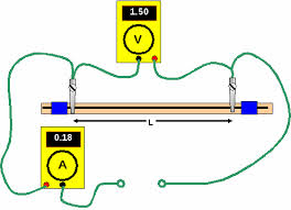 |
A laboratory rheostat is just a long piece of wire wound around an insulator. The slider allows you to select any length - and hence resistance - you want. |
Experimental setup. The power source goes between the two green circles at the bottom. |
However, one of the good things about EEIs is that you can extend the experiment to find conditions that give unexpected results. You could look for sources of error. For instance, when the wire is a short length the current will be large and heating will occur. Heating affects resistance and you should be keeping temperature constant. Perhaps you could place the wire in water (in a beaker) to keep it cool but then it may touch itself and give a 'short' circuit. How would you prevent this; maybe with masking tape, maybe winding it on to a plastic rod so the turns don't touch. You'll want to calculate resistivity so measure the diameter of the wire with a micrometer in several places (does it vary?). Hmmm - this is turning out to be far more interesting than first thought.
Resistance and length of a piece of wire - Part 2
As mentioned in the above suggestion, errors can spoil your results - so why not look at errors in more detail. I'd be taking a length of nichrome wire (which may be 10 ohms per metre) and impressing a voltage across the ends and measuring the current through it. Then I'd try five other lengths. Sounds simple but therein lies the danger: you may overlook sources of error. Be careful if you change the scale on the meters, and remember that the connecting wires have their own resistance anyway - so keep them short (or measure their resistance and include it in your analysis). Finally, remember that the meters themselves have internal resistance. This may not matter unless you are dealing with small resistances - but it may be worth considering. If you know (or can work out) the internal resistance of the meters you can treat them as a circuit component and include the value in your analysis. Voltmeters have high resistance and this would act as a resistor in parallel to your wire; ammeters have low resistance and they would be in series. Voila!
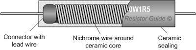 |
 |
Cut-away of a wire-wound resistor |
Big wire-wound resistors can dissipate 1000W of heat whereas other types may only be able to handle much much less. Reference: directindustry.com |
Resistance and length of a piece of wire - Part 3
You could investigate different diameters of nichrome wire as another variable in factors affecting resistance. The resistance should be inversely proportional to diameter as the well-known formula suggests - so it is just a matter of getting some different diameter wire.
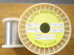 |
| Nichrome wire is pretty cheap and you can all different diameters. |
It may be tricky keeping the length constant as you will probably use alligator clips. Can you improve on this? Will big lengths give you more accuracy? If you measure the diameter of the wire with a micrometer in several places you may get a small variation. Then in your analysis you could discuss measurement errors and the uncertainty of measurements in detail. You may even like to present your diameter data showing the standard deviation of the results.
Resistance vs length: coiled and uncoiled
Because wire-wound resistors are coils they have more undesirable inductance than other types of resistor, although winding the wire in sections with alternately reversed direction can minimize inductance. For the most demanding circuits, resistors with Ayrton-Perry winding are used. If you want to investigate this you may find no difference if you are just using a standard laboratory DC power supply. But if you want to really get in to this you may like to find out about using a high frequency alternating voltage such as that produced by a signal generator. A good (free) computer-generated one is Audacity. You'd have to work out how to measure the input and outputs across the different resistor wire (wound and unwound) and how to analyse the results. This would be quite a demanding EEI but could be very rewarding. It is like the work they do in Physics experiments at university. Good luck.
Resistance and coil types
The suggestion above seeks to compare a straight length of wire with a coil. But you could compare two different types of coils. The Ayrton-Perry winding is a special type used in many electronic components where low values of parasitic inductance and parasitic capacitance ('parasitic' means 'unwanted'). Ayrton-Perry windings of resistance wire are used to make wirewound RF (radio frequency) resistors that are used at high frequencies, where inductance and capacitance are a problem.
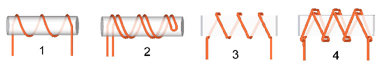 |
| Types of winding used in wire resistors: 1 - simple (inductive), 2 - bifilar (low inductance), 3 - simple on a flat former (inductance reduced due to small cross-section area), 4 - Ayrton-Perry winding on a flat former (the wire is split and wound around the former in opposite directions). Reference: Zureks, Wikipedia |
The winding is made of two separate wires wound in opposing directions along an insulating form and connected in parallel at the ends. There are the same number of turns of wire in either direction, so the magnetic fields of the two wires cancel each other out. Because the coil has little inductance; and since adjacent turns of the two wires are at approximately the same voltage, there is little parasitic capacitance. Other windings are shown in the diagram below.You would need a setup as in the suggestion above (high frequency alternating voltage). You could look at how the output differs to the input at different loads. Changing frequency is another variable but this is getting into waters way past Senior Physics. Tread carefully.
Resistance is Internal - the secret life inside a battery
The chemicals that make up a dry cell have a resistance of their own. It is called "Internal Resistance". When you connect a cell to a load, the electrochemical energy produced by the cell reactions is "used up" in the load and in the internal resistance. We can imagine a circuit made up of a cell and a load resistor looking like this:
When the cell delivers current, the measured emf (voltage output) is lower than the no-load voltage; the difference is the voltage (the product of current and resistance) drop caused by the internal resistance. Hence, a dry cell can be modeled as a voltage source in series with a resistance. The internal resistance of a battery is dependent on the specific battery's size, chemical properties, age, temperature and the discharge current. It has an electronic component due to the resistivity of the battery's component materials and an ionic component due to electrochemical factors such as electrolyte conductivity, ion mobility, and electrode surface area. Measurement of the internal resistance of a battery is a guide to its condition (when it is run down the internal resistance is greater).
 |
 |
| Schematic showing how the internal resistance can be modelled as a circuit component next to the battery (source of EMF). | The load resistance can be provided by a rheostat (the device at the back). It is a variable resistor with a slider that makes contact with the turns of a coiled resistance wire. Photo: http://www.hsphys.com/intresb.jpg |
The internal resistance of a battery can be calculated from its open circuit voltage, voltage on-load, and the load resistance. It is really just a matter of measuring the open circuit voltage (sometimes called the terminal voltage) and the voltage under load. If V = E - IR you can just plot terminal V against I you get Rint as the slope.
Internal Resistance and Temperature
In some of my EEIs, students found that a new alkaline AA dry cell drops from about 0.2W at -10°C in a freezer, where the low temperature reduces ion mobility, to about 0.15 Ws at room temperature and about 0.1 W at 50°C. There's a good idea for an EEI: investigate how internal resistance varies with temperature. Of course the controlled variable would be load resistance. EEIs are about extending your understanding of phenomena to less familiar situations. Perhaps you could try some extreme temperatures for your cell, say dry ice at -78.5°C. I wouldn't be game to try liquid nitrogen (-196°C) or heating it too far (boiling water may make it split open). Nevertheless, what a great experiment.
Lightbulb - brightness and voltage
You may have noticed that when you increase the voltage of the light bulb in the ray box of an optics kit the bulb gets brighter. These are tungsten filament incandescent bulbs. It makes sense: higher voltage means more energy per coulomb of charge going through the bulb - so it heats up more and looks brighter. But this energy is being used to produce heat in the filament and a wide spectrum of electromagnetic radiation.
 |
| A 12 V bulb powered by a car battery at Moreton Bay College. You should try to use the good Senior Physics DC power supplies that have a low ripple. The ones used in Junior Science are often just rectified and have a large ripple. A battery avoids these problems. |
What fraction of the electrical energy is converted to visible light is anyone's guess. It would make a great EEI. Wikipedia says that for a supply voltage V near the rated voltage of the lamp the light output is approximately proportional to V3.4. Why to the power of 3.4? That's for you to confirm. Just change the input V, measure the current, and measure the light output with a light dependent resistor. You'll need to convert the LDR reading into a light intensity value (but there are calibration charts for this). Light intensity is expressed as lumens (lm). The 'efficacy' of a bulb is a measure of how much light is produced per watt of electrical power. It is expressed as lumen/watt (lm/W). For example - a 5W bulb may produce 20 lm so its efficacy is 4 lm/W. If I was going to do it I would start with say 2V and put the LDR next to the bulb. Then I'd increase the voltage to 4V and move the LDR away until the reading was the same. Apply an inverse square law to get a relative intensity to the first one. Note: don't try anything with 240V. You won't get it past your teacher on safety grounds. Stick to car tail-light bulbs (12V).
Lightbulbs - a non-ohmic device
An incandescent light bulb with a tungsten filament has a positive temperature coefficient, and therefore has a very low initial resistance when it is turned off and is cool. As the voltage is increased the filament heats up and its resistance also increases (that's what 'positive temperature coefficient'' means).
 |
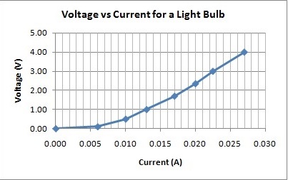 |
| Light bulb measurements at Our Lady's College, Annerley. | Student's results. Using Excel, the graph was shown to be polynomial with a factor of 2 (ie quadratic). |
A bulb is thus said to be non-ohmic [recall that an ohmic device is one where the current is proportional to the voltage]. So here is your EEI. Increase the voltage applied to a lightbulb and take V and I readings as you go. When you plot the data (V on y-axis, I on x-axis) you will get a upward curve. The slope at any one point is the resistance of the filament at that voltage and temperature. What equation best fits the curve and how can you interpret it? I used a 12V bulb and measured its resistance with a multimeter to be 26.0 Ω. For low voltages (up to 6 mV) the slope of the V/I graph was steady at 26 Ω but then it began to rise as the bulb heated. The polynomial trendline in Excel gave a perfect fit (V = 4436.9I2 + 25.8I). If you know the temperature co-efficient (alpha) for tungsten you could hazard a calculation of the temperature at each voltage. What a terrific EEI.
Lightbulbs and heat output
As mentioned above, the energy supplied to a lightbulb from an electrical power source is converted into light and heat. Sometimes you want the light and no heat (as in a torch); other times you want heat and light (in a bathroom heat lamp or the hot-food display at a take-away shop).
An electric torch bulb has a filament - usually tungsten - that glows hot when electrical charge passes through it under the influence of an applied voltage. The filament is enclosed in an evacuated transparent glass vessel that protects the filament from oxidation. The filament is designed so that under a suitable applied voltage - usually in the range of 3V to 9V - the resistance is such that a large amount of "joule" heating occurs. This heat raises the orbital electrons in the tungsten to higher energy levels and when they immediately fall they give off electromagnetic radiation. The frequency of the radiation coming off the filament is quantified by the Stefan Boltzmann Law.
For a typical hand-held torch operating at say 6V DC, the mixture of frequencies should be such that the colour appears white to the eyes. At low voltages - and hence low filament temperatures - the filament glows a dull red, but as the voltage is increased, the temperature also increases. This increased temperature not only produces "whiter" light as more of the blue end of the spectrum is added to the red/yellow frequencies already being produced, but also increases the resistance. For a normal 6V bulb with a cool resistance of say 25 ohm, this increase may change the resistance to many times that value at the operating temperature of 5000 Kelvin (which appears as 'white' light).
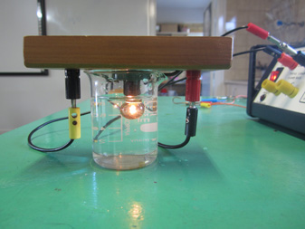 |
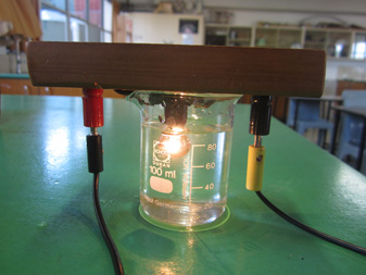 |
A polystyrene cup would be better but a beaker has been used to also measure the light from the glowing bulb. Setup as used at Our Lady's College, Annerley, Brisbane. |
It will keep warming the water until it reaches an equilibrium with the external environment. But you could just measure the temperature change over a measured time so that it doesn't warm up too much. |
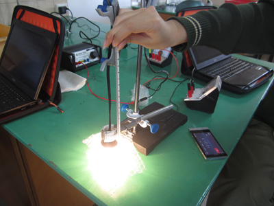 |
 |
| Year 12 Physics students Leanne, Arshdeep, and Anita at Our Lady's College, Annerley, used the 12V bulb from a ray box (optics) kit. Worked well. | Here's the same bulb at a lower voltage and you can see how they insulated the plastic cup of water with bubble wrap. |
The purpose of this experiment is to investigate how the amount of radiation changes as the voltage is increased. A certain amount of the radiation will be absorbed by the water as heat. This heat is wasted in the sense that it is not going into visible light which is the purpose of the light bulb. So what you are looking at is how the electrical energy in is converted into radiation (both visible white light and wasted heat) and how the proportion of these changes with voltage. You are using the temp change of water as a measure of wasted heat. If you put the glass part of a bulb in water and measured the change in temperature for a given time you would have a measure of the heat output of the bulb (Q = mcΔT) for a given energy consumption (W = VIt). The rest is probably electromagnetic radiation. Just change the voltage and measure the heating of water for a given time at different voltages. Does the proportion of energy appearing as heat change as the voltage is increased? If so, why?
The girls at Our Lady's College found that at 4V, only 7% of the energy went into visible light (93% to heat); and at 12 V the light had risen to 22%. But there were lots of problems on the way.
Magnetic Braking I - sliding down an incline
Magnetic braking relies on eddy currents. An eddy current is an electrical phenomenon discovered by French physicist
Léon Foucault in 1851. It is caused when a conductor is exposed to a changing
magnetic field due to relative motion of the field source (eg a magnet) and
conductor. For example, when a permanent magnet moves over a sheet of metal
(such as aluminium), eddy currents are set up in the metal (Faraday's Law) and these can act as
a brake on the motion (Lenz's Law). If you let a magnet slide down an incline on
a sheet of aluminium foil then perhaps the braking current may be observed when compared
to a control. A sheet of OHT plastic on top of the alfoil will keep it from
tearing. But what if you use two sheets of alfoil separated by plastic? Or what
if the alfoil is doubled in width; or twice as thick, or if the metal had higher
resistance, or the speed was slower, or faster, or the foil
was slotted? Oh, the possibilities!

Magnetic braking II - model car
The experiment described above can be varied to consider magnetic braking
of a toy car. The materials I used were a simple toy car, a magnet, a slab
of dielectric material (wood or plastic) and another one of a non-magnetic metal
(aluminium or copper). The magnet used was of neodymium iron boron (NdFeB),
which had been removed from a broken computer hard disk drive. The high level of
magnetic field created by these magnets makes it possible to create interesting
demonstrations of electromagnetism and electromagnetic induction and a beaut
little EEI. Fix the magnet to the underside of the car with
a rubber band and let it run down a wooden incline, and then compare it to
motion down an aluminium incline. It will be slower because of the magnetic
braking. But how much slower. As it speeds up is the breaking force still the
same. Will it be less if the magnet is further away? If so, does it obey some
inverse square law. Oh what fun.
Magnetic braking III - rolling magnet
A neat experiment in magnetic braking is to roll a supermagnet down a aluminium
channel and compare its motion when a non-metallic (plastic or wooden) channel
is used. I've tried it and it works like a charm. However, I wonder if the
braking force is related to the speed of the magnet (if so, why?) and this could
be investigated by varying the angle. There is a little bit of friction with the
walls of the channel but this would be similar for the non-metal and possibly
could be calculated as it would be common to both. Would cutting slots in the
channel make any difference? If you think so you'd need to work out why and
justify your conjecture first. The bait cast fishing reel in the photo below is
one that uses magnetic braking to prevent backlash when casting. It provides
some sort of counter torque.
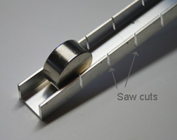
Magnetic braking IV - supermagnet pendulum
Another suggestion is to investigate a supermagnet pendulum. If a pendulum
is allowed to oscillate between two pieces of aluminium (or other non-ferrous metal) the
eddy currents should slow it down. But you'll need to find out if the period of oscillation changes. Some people also measure the 'decay time' - that is the time taken for the amplitude to decay to 1/e of the original amplitude. You could pose the question: does the period and/or decay time vary with the amount of aluminium, or perhaps with the distance between magnet and aluminium. You could compare a freely swinging magnet
(as a control) with the same one swinging as in the photo - between two aluminium slabs (I used
two hotplates on their sides but I could detect some attraction to some hidden
iron). One difficulty is coping with terrestrial magnetism which loves to
interfere. Some variables: length of string (related to period and hence speed),
distance between plates. I had a good time with this until the bell went for the
end of lunch.
Magnetic braking V - supermagnet pendulum
A variation on the experiment above is to lay a sheet of aluminium flat on the bench. Then let the magnet swing over the aluminium and watch it come to rest quickly. Probably best to use a long length of string so that the distance between magnet and aluminium is fairly constant as it swings.What will your independent and dependent variables be. There are a lot to choose from.
Will the manipulated variable be thickness, width, separation distance, type of metal (compare aluminium and copper and see if any variation is related to resistivity), release angle, length of string and so on. For thickness, you could try aluminium foil (1 sheet, 2 sheets and so on) but you will probably need some thicker pieces. What will be your dependent variable: period, amplitude/time graph, decay time (see above)? If they do affect any of these, is there a linear relationship or exponential, or something else? Perhaps you could use a data logger to measure displacement (amplitude) so that you get a heap of data points for analysis.
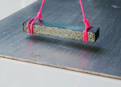 |
An old bar magnet has a noticeable decay in amplitude when swung about 1 cm above a sheet of aluminium. A supermagnet would be even more dramatic. |
This is a great EEI as it has practical uses in industry, domestic appliances, sporting equipment, and in measuring devices; is fairly easy to set up, gives a lot of data for analysis, and can be done at home.
Forces of an rolling magnet
When you roll a cylindrical magnet down an inclined plane, it is
deflected to the left or right from its original direction depending
on the initial orientation of its poles with respect to the Earth's magnetic
field (see diagram below). A good EEI would be to get a sheet of non-magnetic
material (why?) - such as a sheet of plastic or wood and clip a sheet of paper
to it with a line drawn down it's middle. Raise the board to a measured angle
and let the magnet roll down, noting it's path, and the orientation of the board
with respect to the earth's field. Reverse the magnet and try again. Try
different angles and different orientations. What a fabulous EEI. Moments of
inertia of a solid cylinder, and the formula for torque may help.

Measuring the Earth's Magnetic Field Strength
A century ago, the Earth's Magnetic Field Strength (B) was measured by observing
a suspended bar magnet oscillate in a horizontal plane. A new device was
invented whereby a coil of wire was spun in different directions and the voltage
noted. You could try this and get some interesting results. The bigger the coil,
or the more turns, or the faster it is spun - the greater the voltage (Faraday's
Law). You could make a big one out of wood like in the photo below, or make one
out of a plastic fishing reel (below) with an axle glued in place and spun by
hand or in an electric drill (with care). You'd have to work out how to hook up
the moving coil to a stationary voltmeter. And how would you measure the speed of
rotation: stroboscope, stopwatch? There is a formula E = Eo + 2πNAB/T
which has the form y = mx + c and can be investigated (plot E vs 1/T to get the
slope 2pNAB). You
would have to try spinning it in different directions to see how B varies with
the angle, and with speed. A fun EEI if ever I saw one.
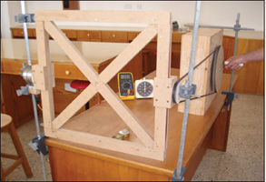
Crash Cushions
Crash Cushion (or Crash Attenuators) are rubber devices that protects the motorist from a
blunt object such as concrete wall or guard rail. Inside of the cushions is a
very high density foam. As the vehicle hits the front of the system, the
system collapses and these devices cushion the impact; like an accordion. You
could model a barrier and decide on optimum type of material and size.
Variables: perhaps force vs. compression, deceleration vs. thickness, mass of
vehicle vs compression. Look at KE, momentum, impulse, spring constant.
Medical physics - blood oxygen and altitude using a
pulse oximeter
Here's a difficult EEI that may be of interest
if you are thinking medical physics. It looks at the changes in blood oxygen
with altitude using a device called a "pulse oximeter" - a clip-on sensor used
in hospitals to monitor oxygen saturation in the blood. You'd have to have
access to one of these. The body is remarkably effective at maintaining blood
oxygenation at a constant level, typically between 95 and 100% (meaning that
arterial blood is carrying between 95 and 100% of the maximum amount of oxygen
that it can possibly carry). However, if you climb a mountain, it is found that
blood oxygenation levels reduced by 6% per 1000 m of ascent.
Pulse oximetry is based on the different absorption spectra of oxygen-rich oxyhaemoglobin and oxygen-poor deoxyhaemoglobin at red and near infrared wavelengths. It exploits this difference by shining two wavelengths of light, one red and one near infrared, through tissue and measuring the resulting light intensity. Two light sources, usually LEDs at wavelengths of around 650 and 900 nm, are held at one side of a convenient site (typically the finger or earlobe in adults, or the foot in babies) and a photodetector held opposite records light transmitted though the body. So, if you are planning a skiing or hiking trip with a group of people you could measure O2 levels at different altitudes, across a wide range of people (different ages, skin colour, weights) and see what you get. Developing and testing an hypothesis is the main challenge. Look at the criteria for your EEI and see how you may meet them. See Physics Education 2009, V44 (6), p 577.
Surface Tension of liquids
You've seen examples of surface tension in action: water striders walking on
water, soap bubbles, or perhaps water creeping up inside a thin tube. Surface
tension is defined as the amount of energy required to increase the surface area
of a liquid by a unit amount. So the units can be expressed in joules per square
meter (Jm-2 ). You can also think of it as a force per unit length,
pulling on an object. It can be used to explain why sap rises in trees, how the
surfactant works in our lungs and why waterproofing agents work. You could
construct a simple balance to make some measurements (see below). Your EEI could
look at how surface tension changes with concentration of solute (eg soap) or
with temperature. If you choose to compare the surface tension of different
liquids then you'd have to have a reason (in terms of physics principles) for
doing so.
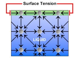
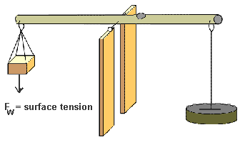

Coupled pendula -
metronomes on a skateboard
I've never tried this but I've been told it works. If you set two metronomes
to the same frequency and place them on a skateboard (or a base that is free to
move), they will not be synchronised and will get out of step. However, if you
wait long enough they will synchronise and become 'phase locked' or 'mode
locked' as they are forced to endure the driving force of each other. Biology
abounds with examples of synchronization: cells in the heart beat together,
audiences often applaud together, fireflies in South-East Asia flash in
synchrony, cicada emerge together, etc.
The earliest known scientific discussion
of synchronization dates back to 1657 when Christian Huygens built the first
working pendulum clock. Huygens studied systems of two pendulum clocks mounted
on a common base. He observed that the clocks would swing at the same frequency
and 180 degrees out of phase. This motion was robust, after a disturbance the
synchronized motion came back in about half an hour. Huygens spent some time
exploring this curious phenomena. You could
investigate what starting conditions are necessary for phase locking. Maybe
start with presstisimo (208 Hz) which is the fastest setting and make
them 180° out of phase. No more hints but you should see the amazing demo on You
Tube:
http://www.youtube.com/watch?v=W1TMZASCR-I
Doppler Effect of source moving in a circle
The rise and fall in pitch of a sound source as it move towards and
away from you can be simulated using a small 9 volt buzzer (from Dick Smith) and
battery attached to a rotating platform. I've seen a 100cm aluminium bar
attached at it's centre to a small electric motor. If the buzzer is at one end,
the battery in the middle and a counterweight at the other end, you'll have
endless fun. Fix a microphone to the benchtop 50 cm from the motor. Record the
sound at rest and then at different speeds. Analyse using spectrogram software
easily obtainable on the web (eg Audacity). Does the Doppler formula
agree with the results. If not, why not? Would something generating a pure
tone be better (eg an iPhone audio function generator app). Does the accuracy
of the formula depend on frequency? Feedback on this EEI comes from
Rachelle East from Genesis Christian College, Bray Park, Queensland: "A
group of my girls last year did the Doppler effect experiment. It was a
fabulous one to do".
 |
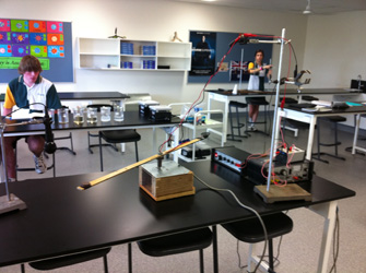 |
| Doppler setup. | Joel Goodwin and Paige Kurmass work on their Physics EEIs in the lab of Katrina Manz at Thuringowa SHS. Cody Gilchrist's Doppler Experiment setup is on the front bench. |
Doppler Effect of source moving on a
pendulum bob
Similar to the one above but with the buzzer attached to a 9V battery -
making a good pendulum bob. You
can calculate the speed mathematically at any point on it's journey by relating
the change in GPE to KE (mgh = ½mv2)
and calculating h by simple trigonometry. A long string
may be better as the period is longer. Of course, the bigger the amplitude (q)
the higher the speed.
Some students have found that the frequency shift is too small to
measure, but by a careful use of a sound sampling program (I find the
free-to-students "Soundcard Scope" digital oscilloscope works pretty well).
I tried with a 2.3 m string and an angle of 30º and got a frequency of 4022 Hz at the maximum speed (at midpoint) for a buzzer that emitted a main frequency of 4002 Hz at rest. The Doppler formula suggested I should have had a frequency of 4030 Hz so I was a bit out. However, that was just one try and I think it could be improved. One other suggestion (but untried) that might help is to record the sound with two microphones: one perpendicular to the plane of swing and a fair distance away (constant frequency providing the displacement is not too large) and one underneath the midpoint of the bob as shown in the diagram below; and superimpose the resulting waves using Audacity. The beat frequency will provide the Doppler shift.
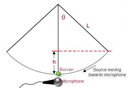 |
 |
| Hold the buzzer "bob" to one side and allow to swing towards the microphone. Capture the frequency as the bob passed over the top of the microphone. You can work out the bob's speed with simple conservation of mechanical energy formulas. | When I found that the main frequency of this buzzer was 4002 Hz, I set the bandpass frequency filter of the "Soundcard Scope" program to a low of 4000Hz and a high of 4050Hz to eliminate other confusing frequencies. |
The Large Amplitude Pendulum
Speaking about pendula, the formula for a small amplitude pendulum T =
2π√(l/g) has to be modified when a larger angle (eg up to 90°) is used. The
modified formula can be found in newer university physics texts and on the
internet. However, you could investigate the effect for yourself and see if
the modified formula really is an improvement. Just remember that the
approximation sinθ = θ when the angle is in radians. One hypothesis could
start "if the
release angle is increased then the accuracy in measuring 'g' will
............ when the mass of bob and the length of the.............are
kept...............".
Simple Pendulum - feeling the Tension
To measure the period (of one oscillation) of a pendulum accurately, you
usually measure the time for 10 oscillations and divide by 10. When your
manipulated variables are length (L) or mass (m) you make angular
displacement (θ) a controlled variable. However, this is a bit of a lie as the
angular displacement decreases with every oscillation - it is not constant. I know it is not
much but could be a significant source of error. It comes about from the
friction of the bob in air, and, of the friction between chains of molecules in
the flexing (bending) of the string or nylon fishing line at the top.
The intramolecular forces between nylon polymer chains in nylon 6, 6 are the quite strong hydrogen bonds so the loss of energy could be significant. But as you know from your study of SHM, the forces on the bob are not constant - they are the least when the bob reaches it's maximum displacement (see figure below). So if you could measure the tension (T) in the string with a force sensor and capture the data with a laboratory interface, a plot of force vs. time should give you the peaks that you need. I won't say any more; this could be a great EEI.
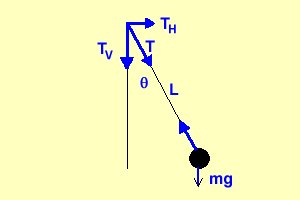

Optimising a solar water heater
Build a model from designs you can find on
the internet; determine what you are going to measure (rate of temp increase
perhaps), then optimise or at least determine the effect of changing various
variables (area, number of tubes, paint colour (gloss vs. matt), glass thickness
(one sheet, two sheets etc). You should be able to hypothesise what the changes
will do to the measured variable. Are there any mathematical relationships? Are
any unexpected? Watch that your controlled variables (eg sunlight) really is
controlled.

Variation in soil temperatures with depth
You may have seen people living underground in
hot place. For instance at Coober Pedy, the hottest place in Australia, the
locals have made their homes beneath the surface as the soil remains cool. Even
when the outside temperature reaches 45°C,
the inside stays about 21°C.
The daily variation in radiation experienced by a soil surface causes the
temperature at the surface to vary widely during the day. The radiation level
will change with the angle of the sun, at night, during cloudy days, during
rain, or in different seasons. This is called diurnal (daily) variation. But the
fluctuations beneath the surface are another thing. The extra time taken for a
particular depth to reach maximum temperature is called "phase delay".
A great EEI would be to look at the fluctuations at various depths (0 cm, 10 cm and so on) as a heat source is applied and removed at the surface. Maybe get a plastic pipe, drill holes every 10 cm or whatever, fill it with the soil being investigated, stick some thermometers in (or temperature probes) and place a heat lamp at the end and turn it on for 30 minutes and then off for 30 minutes and so on. If you had a datalogger and a electronic timer for the lamp you could leave it go for a few days. You get a square wave of heat - but that's okay. Soil scientists tell us that the rate of change of temperature at any depth is proportional to the second spatial derivative of the temperature profile (but that is way to complex for Year 12, and me).
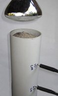
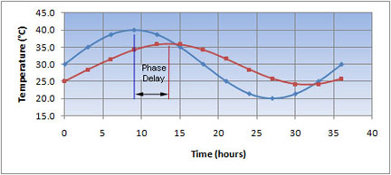
Concrete hydration
The importance of concrete in modern society cannot be overestimated. Look
around you and you will find concrete structures everywhere such as buildings,
roads, bridges, and dams. There is no escaping the impact concrete makes on your
everyday life. Concrete is prepared by mixing cement, water, and aggregate
together to make a workable paste. It is molded or placed as desired,
consolidated, and then left to harden. Concrete does not need to dry out in
order to harden as commonly thought. The concrete (or specifically, the cement
in it) needs moisture to hydrate and cure (harden). When concrete dries, it
actually stops getting stronger.
Concrete with too little water may be dry but is not fully reacted. The properties of such a concrete would be less than that of a wet concrete. The reaction of water with the cement in concrete is extremely important to its properties and reactions may continue for many years. You could make up thin slabs of concrete in a shallow trough with different amounts of water and test their breaking strain. What if you were unable to get fresh water - would seawater be just as good? The possibilities are endless.
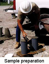

Hysteresis and rubber bands
When you stretch a rubber band and then let it go, you can notice that the
band does not behave like a spring. A rubber band, made of latex and rubber,
does not return to its exact original shape after being stretched. This is an
example of a phenomenon called hysteresis. Small vehicle suspensions using
rubber (or other elastomers) can achieve the dual function of springing and
damping because rubber, unlike metal springs, has pronounced hysteresis and does
not return all the absorbed compression energy on the rebound. Mountain bikes
have frequently made use of elastomer suspension, as did the original Mini car.
By studying the relationship between the rubber band during stretching and
unstretching as weights are added or removed, you can determine the amount of
work done on the rubber band, the amount of energy (in joules) lost by the
band and plot a hysteresis curve. Of course, you'd need more than one rubber
band.

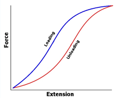
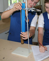

Buckling Height
Galileo pointed out in 1637 that an animal's
bones must be proportionately stronger, therefore thicker, in a large land
animal if they are not to be crushed by the animal's own weight; hence the mass
of the skeleton must rise relatively greater than body mass. This is also of
concern in the growth of trees and in the design of vertical beams for buildings
(eg cylindrical piles). You could investigate how the strength of a hollow
cylinder varies with diameter when keeping the mass and length the same. Maybe
use cylinders of rolled-up A4 paper and look at crush loads for different
diameters and configurations (cylinder, oval, sqaure, rectangle).
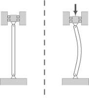

Pressure/Depth Sensor
The deeper you go into a liquid, the greater the pressure on you from the
surrounding liquid. This is the principle behind the depth charge - an
anti-submarine weapon intended to defeat its target by the shock of exploding
near it. Most use explosives and a fuze set to go off at a pre-determined depth.
Would it be possible to design and build a device (not a bomb, just a sensor)
that responds to increasing pressure with depth and a LED turns on at set
depths? You'd have to figure out a pressure sensor and then try out a model in a
swimming pool. It sounds very hard but could be a great EEI.

The Gaussian Gun
If you arrange several steel ball bearings
and a strong (Neodymium) magnet as shown in the picture, you are on the way to
constructing what is called a Gaussian Gun. When a single ball bearing (far
left) is given a gentle push it is accelerated towards the magnet (the the attractive magnetic force) and strikes it
at high speed. The ball to the far right shoots off at a much higher speed. Why?
That's for you to work out and what factors are involved. If the final ball the
strikes another set of magnets and balls mayhem ensues. There are many factors
to examine here: but the number of balls on the right, and the number of stages are worth examining as possible independent variables. How to measure things - that's the question. My students used a LabQuest with Vernier photogates and these worked well. Have
a look on You Tube to see some in action.
The most common approach for students, including mine at Moreton Bay College, is to look at the change in speed of the balls as they go though successive stages of a Gaussian Gun. The KE added at each stage should be the same so the velocities at each stage should increase in a predictable fashion. There are some errors that creep in but these can be dealt with. The second popular investigation is to compare 2, 3, or 4 balls on the right-side of the magnet.
 |
Ball A rolls in slowly and is attracted to the magnet of Stage 1. The energy is transferred through the balls and Ball C flies off at higher speed. It slams into the magnet of Stage 2 and Ball E flies off at an even higher speed. And so on...... |
Theory: There are two possible energy states for a Gaussian Gun consisting of two balls attached to a magnet. See Figures 1 and 2 below. Figure 1 is the "high" magnetic potential energy state. When a ball strikes this combination from the left, the rightmost ball shoots off at high velocity - in fact at a much higher velocity than the incoming ball had. Where does it get this KE from? It comes from the loss of magnetic potential energy (U) of the 'magnet and ball' setup. This is difficult to envisage but I think of this way: It takes a certain amount of energy (work) to remove the outer ball in Fig. 1 (to infinity, say 1 m for this sort of investigation). However, it requires a lot more energy to remove the ball in Figure 2 to infinity. At infinity both balls have the same energy (by definition) so Ball 1 must have had more energy to start with than Ball 2. So there is a loss of energy (ΔU) from Fig. 1 to Fig. 2. This energy is transferred to the ball as KE, and thus it speeds up. Simple huh?
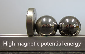 |
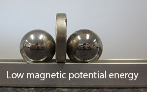 |
| FIGURE 1: It is difficult for students to appreciate that this is the high magnetic potential energy state. It requires just 4 N of force to remove the outer ball. Compare this to the ball in Figure 2. When the ball is removed in either photo they have the same final energy (actually it is said to be zero J at infinity). | FIGURE 2: This is the low energy state. Because the ball bearing is so close to the magnet it requires a lot of effort to pull it away. In fact, it took me 12 N (using a spring balance) to pull it off the magnet. But it requires only about 4 N to pull the ball away in the other photo, so it (Fig. 1) must have had more energy to start with. |
To work out how much energy (work) is done in removing the ball in Figure 1, I just glued a piece of copper wire to the ball and measured the force (on a spring balance) needed to separate it from the magnet (held firm with a zip tie). Then I separated the ball and magnet by 2 mm (with a few bits of plastic) and tried again. And then with 4 mm separation, and then 6 mm and so on. I did the same for the setup in Figure 2. To calculate the work done is very complex but boils down to a simple equation. The relationship between force and distance for a magnet and ball is an inverse square one (y ∝ 1/x2), or Force (F) ∝ 1/r2, where r is the radial distance from the magnet. Here's my plot of the data I got when I did this in my lab at Moreton Bay College (Figure 3):
 |
|
FIGURE 3: a graph of Force vs separation distance (r) for a ball and magnet in configurations as shown above (orange is Figure 1, blue is Figure 2). The constant k is 432 N m2 and 144 respectively. This will be different for your setup. Don't cheat and use mine as it won't make sense and you won't get an "A". |
This video clip shows another method for measuring magnet strength. It shows a magnet being pulled away from a steel plate as a means of measuring the magnet's strength. Students Tara, Emily, Krystal and Cassie Edwards wound the laboratory jack down and eventually the magnet broke away from the plate. This is a recognised method using a 90 x 90 mm (3" x 3") steel plate. The lab jack made their life a lot easier. My life, however, got harder as I have to mark this stuff. |
You can linearize these graph in Figure 3 by plotting F vs 1/r2 and you should get a straight line of slope "k". The work done (W) is equal to force x displacement (W = Fs) but this tricky for a case where the force is diminishing as displacement increases. You can't just average. You have to work out the area under the curve. If you are good at Year 12 Maths you can integrate the formula to get an expression for area (see below). If you don't do this sort of maths you can just count squares on the graph paper (it works well). However, to help you out - here's a suggestion: the integral of F with changing r (distance) is written as:
![]()
You can see that it reduces to a simple equation. For my graphs above, I get 50.4 mJ for Figure 2 and 16.8 mJ for figure 1. You may ask "why mJ?" and that's because I worked in millimetres instead of metres. So the change in magnetic potential energy (ΔU) is 50.4 - 16.8 = 33.6 mJ. This is transferred to the ball as kinetic energy. If it was 100% efficient then all of it would go into KE. I saw that some went in to KE, some into sound, probably a bit into heat, and a bit more into rotational KE (I couldn't stop the balls rolling instead of sliding even when the tracks were oiled).
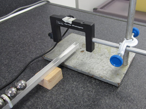 |
|
| Slow motion video of Gaussian Gun in action filmed in a Year 11 Physics class at Moreton Bay College, Brisbane by Cassie Edwards. Three separate interactions filmed at 240fps on iPhone 6. | Sam, Natasha and Chloe's setup at Moreton Bay College. They used a Vernier photogate and LabQuest data logger to measure the speeds of the balls at different stages. |
Students get some great results and plenty to talk about. The errors really show up in the graphs but that gives them heaps to discuss - and this is where they can really show they know what they are talking about. My thanks to Sam, Natasha and Chloe for their reports and hard work.
Fresnel lenses and magnification
Magnification of an overhead transparency on an overhead projector (see below);
dissect an old one with the power cord removed to examine the optics; or open up
a new one; what thickness lens would be needed to replace the Fresnel lens
(pronounced Fr-nell); is magnification related mathematically to the distance
between object, Fresnel lens, top lens and screen?
Strength of spaghetti strands
Spaghetti makes an interesting substance for modelling structures. Three civil
engineering students (pictured below) designed and built a bridge weighing 193
grams that was capable of supporting 53 kilograms. The use of spaghetti is a
great way to demonstrate some basic principles of engineering because it reacts
to the five internal stresses and strains within a structure - tension,
compression, bending, shear and torsion.
For an EEI individual strands can be investigated for their strength by hanging weights on middle of horizontal strand. You could measure displacement ('sag') vs weight for various span widths; or different diameters of the strand. I'm told the sag varies with the weight according to a 4th-power rule; and the diameter vs sag is an inverse cube relationship. But that's only hearsay.


Gyroscope spinning in the
one plane
A spinning object on a moveable axis will keep spinning in the same direction
even if the supports move. The first practical use was for
an artificial horizon in British ships in 1744.
The gyro-compass was invented in 1908. But under what conditions will the axis
remain in a fixed position? What of bearing friction, rotational speed?

The 555 Time Machine
The 555 microchip is an integrated circuit invented by Hans R. Camenzind in
1970 and introduced to the world in 1971. Using simply a capacitor and a
resistor, the timing interval can be adjusted and so can be used for numerous
applications including timers, clocks, switches, security alarms and tone
generators. Circuits are freely available on the internet. An idea for an EEI
would be to test the accuracy of the timing circuit. The problem is - how do you
measure it's accuracy when the stopwatch you would used is based on a 555 timer
anyway? Perhaps you could see if the error is related to the tolerances of the
resistor and capacitor; or perhaps you could make a few of them and see how they
vary; or perhaps you could see how reliable they are with varying temperatures.

Pullling a spool of cotton by a thread
An old favourite: investigate the conditions for rolling forward or backward;
angle; effect of weight and surface friction - see diagram below. Again, why
would you want to know this? Aimee Leong tests this out.
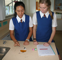

The Kelvin water dropper
The Kelvin water dropper, named for Lord Kelvin (William Thomson), is a type of electrostatic
generator. Kelvin referred to the device as his water-dropping condenser. The
device uses falling water drops to generate voltage differences (up to 6000 V)
by utilizing the electrostatic induction occurring between interconnected,
oppositely charged systems. It is possible to build a very simple high-voltage
generator which has no moving parts. By dripping water through some old soup
cans, several thousand volts magically appear. An EEI would be to investigate
the conditions under which the potential differences appear: size of cans,
distance drops fall, rate of flow and so on.
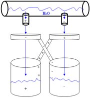
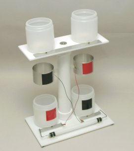
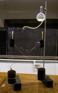
Turbine efficiency
This EEI models a device known as a "fluid coupling" similar in many ways to
the processes occuring in the automatic gearbox of a car. A fluid coupling is a
hydrodynamic device used to transmit rotating mechanical power from one part to
another. It also has widespread application in marine and industrial machine
drives, where variable speed operation and/or controlled start-up without shock
loading of the power transmission system is essential. In essence it
consists of two turbines (fan like components): one connected to the input
shaft; known as the pump, impellor or input turbine. The
other connected to the output shaft, known as the output turbine or just
plain turbine. A good investigation would be to see what factors affect
the efficiency of the conversion of mechanical energy from one fan to the other.
You could do this with air as the fluid, or try it in water or oil (your teacher
may hate you using oil in the lab at it makes one enormous mess and is hard to
clean up). For a more viscous water-based liquid you could start with honey and
gradually dilute it. The photo below uses a low-voltage motor turning a fan to
provide the wind, which blows against another fan to drive a low-inertia dynamo
(the turbine). It is up to you to develop an hypothesis and a way of measuring
input and output energies (perhaps using a voltmeter). An efficiency vs speed
graphwould be fascinating.
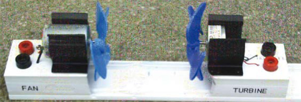
Windpower: the world of carbon reduction.
Wind energy is plentiful, renewable, widely distributed, clean, and reduces
greenhouse gas emissions when it displaces fossil-fuel-derived electricity. It
is considered to be more environmentally friendly than many other energy sources
and worthy of our investigations. Most wind turbines seem to be 3-bladed whereas
domestic fans seem to be 3, 4, or 5 bladed. As well, wind turbines can have
adjustable blade angles. You could make some model turbines hooked up to a small
electric motor and measure the voltage produced when you blow air on it. How
does blade angle, blade length, number of blades etc affect performance?
 |
 |
Are three better than four? |
Need to decrease the pitch in high winds or else. |
 |
 |
|---|---|
| Home-made fan using cardboard blades |
Buy a fan and run it backwards as a generator. |
Yagi Transmitter
A Yagi-Uda antenna is familiar as the commonest kind of terrestrial TV antenna
to be found on the rooftops of houses. It is usually used at frequencies between
about 30MHz and 3GHz, or a wavelength range of 10 metres to 10 cm. You may know
that they are directional and when being installed they have to be rotated until
the strongest signal is found. A Yagi transmitter has a characteristic pattern
of signal strength as shown in the figure below. An EEI that a Year 12 radio
enthusiast from Sandgate State High School (Brisbane) undertook was to study the
radiation pattern of a halfwave 5-element Yagi antenna transmitting a signal
from a 147 MHz VHF
transmitter. Suggested dependent variables are
distance and angle. If this means nothing to you then this EEI would not be
any fun. If you are in to radio communications or know a ham-radio enthusiast then it could be good. The
student was Gal Strasberg (seen below) and his physics teacher was Ewan Toombes.
You don't need to make the antenna - just buy one. And you'd have to buy, borrow
or hire the VHF transmitter and the field strength meter. Gal bought the
transmitter online from a radio communications supplier (Andrews
Communications), and the built the field strength meter himself using a basic
tuned circuit similar to the one at:
http://www.zen22142.zen.co.uk/Circuits/rf/fsm.htm

Yagi Transmitter #2 - Build and test your own
The Yagi antenna shown above is a commercial antenna and transmitter and the student verified the expected pattern. Students at Nanango State High School (Queensland) under the expert guidance of Physics teacher Mr Peter Cavallaro took a different approach. His students designed and built their own antenna, a rather simple one - 3 element Yagi, optimised it on antenna design software and designed their own transmitter on 5Spice (circuit analysis software). Peter admitted it was a huge project design and build, and did not finish in the time frame allowed but is hoping to take further in years to come.
 Peter is an indefatigable champion of physics: amongst dozens of other projects he established an industry partnership with the Meandu Mine to support an advanced computer design program that gives students access to professional industry standard advanced design software and computer controlled manufacturing. Thus, his plans for a Yagi EEI are well worth considering. The photo opposite is of him receiving the Queensland Minerals and Energy Academy (QMEA) Teacher Recognition Award 2010 (and cheque for $4000.
Peter kept his design low-tech so there is no reason any school could not reproduce it. In essence, the Year 11 Physics students built 144Mhz transmitters with a 1kHz audio signal modulated onto it, proved in 5Spice and then designed and optimised a 3-element Yagi on industry standard software with 50dB front to back (F/B) gain, then built it and analysed it on a software defined radio receiver, compared to an Omni-directional whip. He said "it is not pretty but does give a measure of the antenna performance in relative terms".
I was interested that this radio transmission uses the frequencies in an Amateur Radio band. These are not public access frequencies, so any transmission in these bands requires that the person in control has an Amateur Radio licence and the official callsign of the license holder must be transmitted. There are frequency bands where no license is required provided some restrictions are complied with. Some of these are higher frequencies where Yagis are a more convenient size. Peter said that "transmit power is milliwatts and is undetectable above noise at 200m. We have made sure of this by local HAMs tuning in. We are transmitting via a licenced HAM operator."
 |
| Results from directional antenna; max gain @ 0 deg. The software being used is HDSDR (High Definition Software Defined Radio) - download from http://www.hdsdr.de/ |
 |
The result at 90 deg: holy crap - this is some serious forward gain! |
Polarisation. If you are after a high-powered research project for your EEI you could try the following - suggested to me by Steve Hutcheon (School of Engineering at QUT). It is about antenna polarisation. "Polarisation is an important property of all antennas including Yagis. To work best the transmit and receive antennas should have the same polarisation. The polarisation project would be to measure the reduction of signal strength as the antennas become cross polarised. The results can be graphed and an equation found that matches the curve. Polarisation can be used to reject interfering signals or allow a second signal to be used on the same frequency at the same time over the same path."
Yagi-Udi Antenna #3 - proximity of humans
Further to the above suggestions about hypothesis testing of a Yagi antenna: here's a good idea. It has been found that when a person gets close to an antenna the gain can drop considerably. For example, Professor David Thiel from the School of Engineering at Griffith University found that when a person was close the signal gain was degraded by more than 2 dB. He used a 12 element Yagi (1 reflector element, a driver, and 10 director elements) optimised for 300 MHz - but you could just as easily try it with fewer directors. Human proximity has a significant effect on link reliability in RFID (radio frequency identification) and wireless sensor networks where power is restricted. The context for this EEI is thus obvious. You can download his paper here.
 |
 |
| Polar radiation pattern of the Yagi-Uda antenna in free space. (Thiel 2009) | Polar radiation pattern for the same setup as on the left but with a human model on the right side 10 cm of the driven element. |
Theremin Synthesiser
The Theremin is a device that detects changes in the electromagnetic field that
it radiates and by use of clever electronics uses the changes to alter the
frequency of a sound generator. It was used in the construction of the Keck
Observatory in Hawaii. As the Keck's mirror was 4 times larger than any other
built before it, careful alignment of the mirrors was essential. The Theremin
could detect changes in the position of objects down to nanometres.
For an EEI, why not build a Theremin from a kit and investigate what
changes its output? Jaycar Electronics (Aust.) has them for about $60.
The sound is produced by the interaction of two radio frequency oscillators which normally are operating above the range of human hearing. However, if one of these oscillators is slightly detuned by varying it's frequency (by placing objects near it to change the capacitance) while the other oscillator remains fixed, the difference in the frequencies (known as the beat frequency) is in the audible range and can be amplified. This process is known as heterodyning. It is a weird sort of electronic musical instrument that you play by moving your hands in the magnetic field that it puts out. Its definitely a strange sort of gizmo and would be a pretty good thing to keep once you have finished your EEI. You can make all sorts of sci-fi effects like in the old flying saucer movies and the sounds from The Beachboys song Good Vibrations. Click here to listen to some Theremin music on YouTube. WARNING: the important part of your EEI won't be in building it but in using it to test your hypotheses.
String unwinding on a pole
Measure time for n turns; variables: initial length, radius of pole,
angle, weight of bob, speed, amplitude.
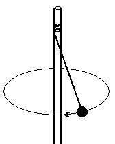 |
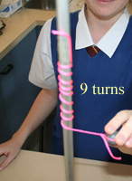 |
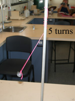 |
 |
| Rebecca (Moreton Bay College) starts it off with 9 turns around the stand. | When 4 turns have unwound (leaving 5 left to go) the amplitude was 10 cm. | When 5 turn have unwound the amplitude is 15 cm and the speed is even greater. |
Kicking a football
Measure time of contact using Alfoil
strips on the ball and shoe as a timing switch; measure time of flight, range,
angle, pressure).

Electric strain gauge
A strain gauge is a device used to measure the strain of an object. Invented in
1938, the most common type of strain gauge consists of an insulating flexible
backing which supports a metallic foil pattern. The gauge is attached to the
object by a suitable adhesive, such as superglue. As the object is deformed, the
foil is deformed, causing its electrical resistance to change. You could compare
one to a length of nichrome wire and measure it's resistance as weights are
added; try parallel; try other wire. Do they behave in a similar fashion? If
not, why not?
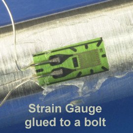
Roller Coaster
Loop-the-Loop
Have you noticed that the loops in a roller coaster rise are not circular; they
are ellipses. The reason is to do with the maximum centripetal acceleration the
body can take before blacking-out. Now, they don't want you to black out as it
would hold up the ride, and you wouldn't be able to go and buy their overpriced
food. Model one using flexible track and try varying ratios (major axis : minor
axis). Vary the speeds; contemplate conservation of mechanical energy. What are
the various combinations of speed and axis ratios needed to keep acceleration
below the safety limit?
Friction: another investigation might be to find the minimum value of the initial speed of an object that is needed to traverse the entire loop. We easily find that the kinetic energy at the bottom of the loop must be equal to the potential energy of the object at its initial position on the inclined plane. The problem becomes more difficult if we consider the existence of sliding friction between the object and the circular track. While you may know that the frictional force Ff = μFn, where Fn is the normal force that the object exerts on the track, but you will soon realise that this normal force varies with the angular position in the loop and that involves the cosine of the angle. All of a sudden is is a difficult problem and would require a bit of calculus to solve it. While it is challenging to analyze not only how the frictional effects influence motion on the circular loop and the conditions for the object to go around it, you wouldn't have to be able to model it mathematically at a Year 11 level. What you would do is collect and analyse the speed and angle data, and try to explain the relationship. Difficult but not impossible. There's a good article in the American Journal of Physics, 79 (9), September 2011, p 913.

Air damping
A 'damper' is a device that eliminates or progressively diminishes
vibrations or oscillations. A shock absorber in a car deadens (dampens) the
up-and-down movement because it contains a dampner called a dashpot which
resists motion via viscous friction. The resulting force is proportional to the
velocity, but acts in the opposite direction, slowing the motion and absorbing
energy.
Vertically suspend a brass 'weights'
hanger from a spring and measure oscillation period as masses added; then make a
cardboard damper and try again. Is decay of period logarithmic? Vary area of
damper.


Modelling sporting equipment as solid pendulums
The "sweet spot" for a piece of sporting equipment is the region of the bat
or racquet which gives players the optimal result from a stroke. It is sometimes
said to be the centre of mass, centre of percussion, the power centre, the area
that gives the most bounce, the are which gives the least vibration to the
holder's hands etc etc. There are twenty different definitions on the web. A
good one to investigate is the centre of percussion (where a perpendicular
impact will produce translational and rotational forces which perfectly cancel
each other out). Another is to model the bat to a solid pendulum. You could make a comparison of a cricket bat, baseball bat etc with metre ruler etc.
Factors affecting the restitution of bouncing ball
The coefficient of restitution or COR of an object is a fractional value
representing the ratio of velocities before and after an impact. But as it is
difficult in the lab to measure velocities you can measure bounce heights and
work out the velocities. Actually restitution in just the ratio of the square of
the heights. You could investigate if restitution decreases as the number of
bounces continues (or just change the starting height). As a matter of interest,
he International Table Tennis Federation specifies that the ball must have a
coefficient of restitution of 0.94. What is the effect of temperature, gas
pressure, mass etc? If you are comparing balls (eg golf vs tennis vs cricket you
would need to know why you are doing this and what you hope to show. The fact
that they are different may be of little interest in terms of physics concepts.
 |
 |
I tried bouncing some foam practice golf balls that had different temperatures. My Moreton Bay College girls plotted the results on the board. They are pretty rough results but it was just a demonstration. The % restitution has been plotted as a function of temperature (in °C). For an EEI you would use Kelvin. |
A strobe flash picture of a bouncing ball. You can easily caluclate the %restitution. Does it vary on subsequent bounces. Who knows. Perhaps the ball heats up and it gets more bouncy rather than less. I wish I was doing this EEI. It looks like fun. |
Friction and temperature
Have you seen racing car drivers spin their wheels before a race to get the
tyres hot and sticky and to increase friction (perhaps)? Just how does
temperature affect friction? Are intermolecular attractions reduced as
temperature increases? A neat little EEI would be to measure frictional force
between two surfaces and then heat them up (in an oven) and measure it again.
Have a look at the nosewheel of this Italian Air Force G222 transport plane at
2002 Riat airshow!

Newton's Law of Cooling - 1
In 1700 Newton published his Law of Cooling (in Latin) which stated that the rate of change of the temperature of an object
is proportional to the difference between its own temperature and the ambient
temperature (i.e. the temperature of its surroundings) when "placed in a wind
blowing uniformly, and not in a quiet Air, that the Air heated by the Iron might
always be carried away by the Wind, and the cool Air might succeed in its
place" [his words]. Most texts leave out the last sentence because of a superficial reading of Newton's report. I checked 17 university Physics
texts at the local University and only one mentioned that the Law only applies in a breeze. Throughout the 1800s physicists also forgot about the breeze
until a physicist at Edinburgh University (Prof. Crichton Mitchell) reviewed the
original in 1887 and pointed it out to shamefaced colleagues.
A good EEI would be to see if
Newton's Law of Cooling applies with or without a breeze. Even better - see if the
strength of the breeze (the independent variable) makes a difference. And what will you measure as the dependent variable? Further, what will you analyse for: the rate of cooling, or the temperature after a set time, or how long it takes to get to room temperature (Newton got 200 minutes to reach body temperature for his experiment)? This knowledge is important today as engineers, for example, need to know rates of cooling of metals when they are designing equipment in which metals are cast. That is, when trying to mould metal items using centrifugal casting the moulds are spun and the rate of cooling depends on the type of metal and on the speed of rotation in the air (acting like the wind). In one example I saw, at 200 rpm the rate of cooling was 16°C per second, and at 400 rpm it was 25°C/s.
 |
An old shotput with a drilled hole
for a thermometer probe might be a good start. But how do you support the metal? Newton didn't think of the conduction of heat through the benchtop but you should. How can you insulate it from the surface? |
Newton it seems was lucky that he heated his metal to the comparatively low (yes, low) temperature of 300°C. He thought that all heat was transferred away from the metal by the wind. We now know that there is also radiation losses given by the Stefan-Boltzmann Law which states that the rate is proportional to the difference between the fourth power of the absolute (Kelvin) temperature of the metal and the fourth power of the ambient temperature. This is not significant when the temperature difference is not high (<300°C) - but that's for you to investigate and say why. This would be a fabulous EEI although I'm not sure how you would safely heat a shotput up to a high temperature.
Newton's Law of Cooling 2
Another good research question (following on from the one above) for an EEI would be to ask if different metals cool at different rates. You might think they would differ depending on the metal's specific heat capacity (high specific heat = low cooling rate).
Newton, from 1700 to 1727, was Master of the Mint in England and responsible for the manufacture of coins. Hot gold plates about 9 mm thick was drawn slowly between two rollers to give it a uniform thickness and then coins were punched out of the metal plate. The problem was that as a plate was drawn through the rollers it cooled and so the last part of the bar had more time to cool than the first part, so the last part shrunk more than the first part and was more dense. The unfortunate result was that some coins had more gold in them than others. He had to know more about the cooling rates of alloys. As coins were made of different alloys, Newton measured the specific heat of various coinage metals and found that copper (with a high specific heat) cools slower than gold (low specific heat). His knowledege of rates of cooling and specific heats helped him solve the coinage problem.
A good EEI would be to investigate the rate of cooling of metals and see if it is related to some other related charactistic such as specific heat or thermal conductivity, or perhaps density. You'd have to justify why the two were related. In your design you would have to decide the temperature range (Newton used 300°C to body temperature); what variables you would control (mass or volume as you can't do both at the same time), or shape. And you'd need to look at all the different ways that objects lose heat. I can think of four (one is to the breeze).
Atwood machine and 'g'.
The Atwood machine was invented in 1784 by Rev. George Atwood as a laboratory
experiment to verify the mechanical laws of uniformly accelerated motion.
Atwood's machine is often used to measure 'g'. But how accurate is it? Surely
the friction in the pulleys would defeat accurate measurement. But perhaps
friction is lower when the masses are lower and maybe accuracy improves. Perhaps
it is more accurate when the difference in masses is great. Who knows. Why don't
you find out?
What is the 'best' way to heat water; kettle or microwave oven?
You'd think that a kettle would be as it is designed to heat water; but the
microwave is more modern and could be better or more efficient. But what is efficiency? What does 'best' mean here? How is efficiency affected
by volume of water; time of heating. Should energy input be kept constant, or
just time?
A rubber band under stretch and relax
Elasticity is an important factor in the design of building frames. For example, what is known as the "hybrid frame" design provides elasticity in response to dynamic loading caused by an earthquake, and the effects are like a flat rubber band held at both ends and stretched. The rubber band will stretch but not break, and then return to its former state. A hybrid frame building reacts much the same way, resisting the lateral forces of the temblor and reverting to a static state after the action stops. You could model the behaviour of this building material using a rubber band and look at a number of factors: how many times can it be stretched; effects of temp; coefficient of restitution vs cross-sectional area of rubber, and so on.
Impact craters of meteorites and tsunamis
When an asteroid hits the ocean at a typical speed of 70000 kmh-1 there is a gigantic explosion. The asteroid and water vaporize and leave a huge
crater - typically 20 times the diameter of the asteroid (that is, a 100 m
asteroid will create a 2 km diameter crater). The water rushes back in,
overshoots to create a mountain of water at the middle and this spreads out as a
massive wave - a tsunami. The centre of the crater oscillates up and down
several times and a series of waves radiate out. You could investigate how
the diameter of the crater relates to the diameter, speed, density, mass of the
meteorite. I think a video camera might be necessary for this. If this is too
awkward perhaps letting objects of different size, mass, speed etc fall into
sand (fine, coarse) might be easier.
There is an interesting article by Michael C LoPresto of Henry Ford College, Dearborn, Michigan, USA in Physics Education 51 (2016) p1-4 titled "Experimenting with impacts in a conceptual physics or descriptive astronomy laboratory". He had his students drop balls of different mass (different metals) from a set height of 10 cm, and also of the same ball from different heights. I tried this (see results below) and achieved similar results. He was predicting an exponential relationship between GPE and crater diameter with the power being 1/3 to 1/4. Mine was D = 0.15(GPE)0.25. You need to use a fair depth of sand (at least 5 cm) and set it in a tray on a hard surface.
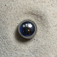 |
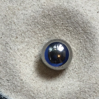 |
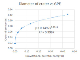 |
Rim diameter 40 mm from an 18 mm diameter steel ball dropped from 20 cm height. |
Rim diameter 56 mm. Same ball dropped from 30 cm height. |
Plot of GPE vs crater rim diameter for different mass balls at a height of 20 cm. |
The angle of a meteor strike and crater shape
Why are impact craters always round? Most incoming objects must strike at
some angle from vertical, so why don't the majority of impact sites have
elongated, teardrop shapes? If you throw a stone into sand on the beach
at even a small angle from the vertical you get an elongated crater; so why not
for real meteors? The answer seems to be that the physical shape and direction
of approach of the meteorite is insignificant compared with the tremendous
kinetic energy that it carries. Elliptical craters may only show up at really
small angles for meteors. However, a good EEI would be to model impact angle
using marbles in sand, or in flour. A layer of cocoa powder on top of the flour
makes it easy to photograph.
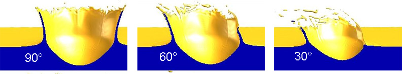
Thermal conductivity
Thermal conductivity, k, is the property of a material that indicates its
ability to conduct heat. It is very important in industry. One interesting way
I've seen is to drop a cube of metal into water in a polystyrene cup and measure
the rate of heating of the water. Seems so simple but is it accurate? Is surface
area important? Doesn't the rate of warming slow down as the difference in
temperature gets less? An interesting application of thermal conductivity
testing is shown below. Here they are trying to get an accurate value of the
existing soil conditions for a geothermal project.
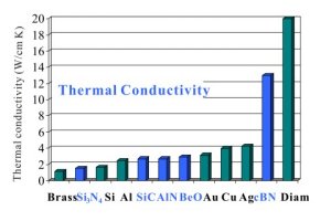

Investigate conservation of momentum and kinetic energy in two dimensions
A good EEI if you like billiard table physics. Measure the effect
of 'English', spin, position struck etc; any access to TI /Casio/Pasco photogates?
This is too much fun to be Physics.
Interference effects of
sound in a room
Audio engineers go to a lot of trouble working out the best placement of
loudspeakers in a room. For example the recommended placement for 7.1
Channel Surround Sound is: Front speakers
should be placed at the edges of the screen, toed in to face the central
listening location, and the tweeters should be ear height. The center speaker
should be placed behind the screen (when using projection) or over or under a
TV, and as close to ear height as possible. Side channel speakers should be
placed on side walls, to the left and right of the listening position,
equidistant from the front speakers and the rear speakers. Rear channel speakers
should be placed on side walls, slightly behind the listening position, and
should have a normal high-quality monopolar construction. Front speakers should
be at ear height and surrounds should be above ear height. See diagram below.
It is even hard enough just getting the placement right for a simple two-channel stereo. A part of the problem is because even a pair of sound sources (speakers) emitting a monophonic sound generate interference in the room - even without considering reflections off the back and side walls. An interesting EEI would be to try one and then two speakers in a room (say left and right front) emitting a pure tone from a frequency generator and measure and account for the nodes and antinodes (as measured with a microphone and CRO). You can decide the controls and manipulated variables (but keep it simple).
Specific heat of metals
It is pretty useless just measuring the specific heat using a calorimeter and
water; that's hardly an EEI deserving of an "A" standard. But if you can
optimise the method and improve it's accuracy then you could be on to a winner.
How do volume of water, initial water temp, mass of metal, size of calorimeter
(copper vs polystyrene foam and amount of insulation affect the accuracy? Are
you going to do it electrically? If so, won't the resistor heat up and change
resistance as the experiment progresses; are you using a stable DC source or a
unfiltered rectified AC source from a lab power supply that is bumpy (see
diagram below)? This may affect your voltmeter reading and the calculation of
energy transferred:
How high will water syphon?
Use clear plastic tube 20 m long in U-shape; effect of boiling water first;
effect of temperature. Is the density of the liquid the main factor or is vapour
pressure or intermolecular force a factor?

Investigate the coefficient of friction for accelerating surfaces
For sliding friction on an incline, the coefficient of friction μ = tan θ for
constant speed; but if the block is accelerating life is not so simple. You
could investigate friction for objects being shot up an incline and
coming to rest (what to vary, what to control?). What about the motion of a
block of wood resting on top of a piece of wood that is oscillating back and
forth?
Egg cooking
The yolk and
white of an egg have different thermal conductivities so I'm told. So how does
the temperature rise of the two parts of an egg compare when it is being boiled.
Much work has been done on eggs but maybe not on this. I'd say you'd need the
temperature probes and a lab interface of some sort.

Investigate the absorption of sound at different frequencies
In the music rooms at Moreton Bay College there are large sliding panels
hanging from the wall. One side of the panel is covered with a loop-pile carpet,
the other side has cork. I asked the architect why he did this and he said so
they could 'tune' the room and remove annoying frequencies. You could do an EEI
to investigate the sound deadening effect of different substances. How does % absorption vs thickness; vs frequency; vs loudness.
What relationship is there with density of the sound absorbing barrier?)

Meniscus shape
Think of how many times your teacher has cautioned you to "read to the
bottom of the meniscus" when you're using a measuring cylinder, pipette or
burette.
A
characteristic of liquids in glass containers is that they curve at the edges.
This curvature is called the meniscus. Think of how many times your science
teacher warned you to read to the bottom of the meniscus when reading measuring
cylinders and so on. How does the meniscus angle change with temperature, type
of liquid (eg various alkanes), density.
Construct and investigate a simple, tuned musical instrument
Which harmonics are emphasised (odd/even); factors affecting the sound envelope
(attack, sustain, decay); how can you modify your instrument to increase the
range of frequencies both higher and lower? As a start, I've measured a school
xylophone but removed some of the key dimensions.
Investigate the speed of sound in air
It is said that the speed of sound increases by 0.6 ms-1 for every
degree Celsius rise in temperature. But is this accurate over a wide range
of temperature change? You could investigate: speed vs temp; vs humidity; speed in different gases (different densities,
molar masses). Or how does it vary from a day of high pressure (eg 1020hPa) to a
low pressure day (eg 995hPa)?
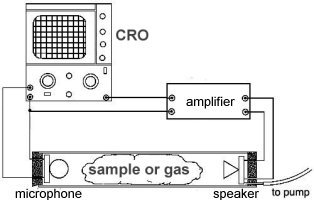
Self-inductance in a
solenoid
Consider the circuit below (left). Nothing happens to the brightness of the
bulb when the metal rod is inserted into the coil. But if you use the circuit on
the right where the source of power is an alternating current, insertion of the
rod affects the brightness. This illustrates the property of self inductance. As
a consequence of this, when a DC supply that is connected to a solenoid and is
switched on, the current doesn't respond immediately. The same is true when the
circuit is switched off. You could investigate the effect of different metal
bars, coil size, size of AC etc. A CRO may be better than a bulb for getting
quantitative data.


Molecular sizes of gases
You know how helium balloons deflate rather quickly as the gas leaks through the
porous rubber? Well, a hydrogen balloon deflates even quicker as it's molecules
are even smaller. You would think that the rate of deflation would somehow vary
with the molecular size.

Measure the audible range of a human being
You could measure frequency range, loudness; may be able to get access to
audiologist's equipment; variation with age, sex, occupation; test family and
friends. But how do you stop it being so subjective. Where does the physics come
in? This would not be a 'manipulated variable' EEI but one that relies on natural variation. It is sometimes called the 'method of concomitant variation' and is more familiar to Biology students than to Physicists. For a Physics EEI you'd have to be vary careful that you were able to demonstrate all the criteria in the task sheet. My advice is to talk to your teacher about it before you get too far into it.
Wing lift
One of the things keeping a plane in the air is lift. Lift is produced by a
lower pressure created on the upper surface of an airplane's wing compared to
the pressure on the wing's lower surface, causing the wing to be "lifted"
upward. The special shape of the airplane wing (airfoil) is designed so that air
flowing over it will have to travel a greater distance faster, resulting in a
lower pressure area (see illustration) thus lifting the wing upward. Lift is
that force which opposes the force of gravity (or weight). You could make models
of wings and place them in front of a fan. Vary the attack angle, shape and so
on. Clue: read up on The Coanda Effect.

Investigate the interference of sound waves
Can a wave be superimposed on another to cancel out the sound? This is what they do in noise-cancelling
headphones and car interiors. Maybe too complicated for an EEI but you could
look at interference of waves between two speakers and measure the degree of
cancellation (but how to minimize reflections off the walls?).

Rate of cooling and surface
area
An interesting EEI can be made from filling balloons of different sizes and
shapes (cylindrical, spherical) with hot water and measuring cooling rates in a
gentle forced breeze. You can look at shape and surface area.

Perpetual motion machines.
Now we know they can't work but trying to figure out why they can't work is a
bit harder. You could make a few models from designs on the internet and work
out what they don't work. You'll need some estimate of % efficiency and that
might be hard to gather.

Variables that affect drag forces in boats.
The "Hull Speed" is the maximum speed
before drag increases dramatically. For a 30m ship it is about 24km/h; for a
30cm duck it is about 2.4 kmh-1. There's lots to test and talk about there. I'm
guessing it's all to do with the ratio of surface tension to hull area.
Variables: drag vs speed; length; width; shape.
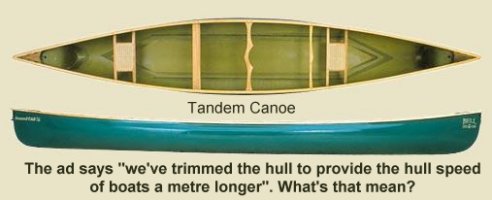
Switching from walking to
running
Prof. McNeill Alexander from Leeds University (UK) developed Alexander's Rule which
says that v2 = gdH/2 (where dH is the distance
from hip to ground) that shows the speed at which an animal switches from
walking to running and this is supposed to work for insects to humans. But I'm
not so sure! How could you do an EEI on this? Better get good advice from your
teacher before you start.
Controlling the speed and direction of sailboats
Hint: collision trolley, sail, electric fan, spring balance; wind force vs
angle, speed of wind, area of sail; say no more!

Does pyramid power really work?
What possible forces; size of pyramid, material, angles, what to test
(freshness of eggs?); is this really science?
DC Motor
What factors affect the rotational speed of a simple DC motor. You'd think that
as you increased the voltage it would just get faster and faster, but alas, a
thing called "back EMF" spoils the party. What factors are involved here?
 |
 |
 |
| Why not dissect one first? | Simple motor | Home made motor from Churchie. Click image to enlarge. |
Mersenne's law
To determine if Mersenne's law of stretched springs
applies to slinkies.
Well why shouldn't it; it is the same principle. But how do you minimize
friction. And what about the heavy spring: snaky?
Factors which affect the
specific heat capacity of various concentrations of salt water solutions.
In a lot of questions you are told to take the specific heat of a solution
(seawater, milk) as being the same as distilled water. But is this fair? Maybe
some of the heat is used to increase the vibration of the hydrated Na+ and Cl- ions. But wait - 100 g of salt water has a smaller volume
than 100g distilled water so maybe......
To measure the specific latent heat of vaporisation
of liquid nitrogen.
The specific latent heat of vaporisation of water is not such a big deal - it
has been done to death by physics students in laboratories all over the world
for the past 140 years. But this is an EEI and critical thinking has to be
applied. That's why nitrogen could be tried. Liquid nitrogen is not easy to get
hold of or store, and even less easy to handle. Doctor's surgeries often have it
to freeze off warts and skin cancers so maybe there's a clue. It wouldn't be
easy but with teacher guidance this could be a great EEI.
To determine the effect of changing temperature on
the viscosity of honey.
Have you ever tried to eat
honey that has been in the refrigerator - hopeless huh? Both the viscosity and
the density of honey change with temperature and water content and I'm told the
viscosity and temperature follow a inverse cube relationship.
Honey is mostly sugar (glucose/fructose and water). Thus the two variables seem
to be temperature and moisture content. But how will you control moisture, and
how will you measure viscosity (maybe a ball bearing - but what size and what
about the diameter of the tube - is there viscous drag)?


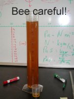
Can a pendulum predict the sex of a chicken while it is in the egg?
Is this really physics?; what forces are acting?; who thought of this? You'd have to be very confident or plain daring to choose this for an EEI. I wouldn't do it.
Can eggs stand more force from some directions?
Build a pressure gauge; can it be connected to a TI-CBL or computer; what is
the hypothesis?. Does cooking (for how long) affect this?
How strong is human hair of different thickness?
For a healthy individual with no hair diseases, hair fibre is very strong
with tensile strength around 1.6 x10⁻⁹ N m-2. That makes hair about
as strong as copper wire of the same diameter. So as you can see hair is
incredibly strong. It also has elastic properties. It can stretch up to 20% of
its original length before breaking when it is dry and when it is wet it may
stretch up to 50% before breaking. But do you believe the ads that say their
products can improve the strength of hair (see the one below). Sounds a bit
far-fetched to me. You could measure elongation vs weight; breaking strength vs diameter; vs colour;
are different colours more stretchy (how to control variables?); effect of
humidity, heat, prolonged light, age of subject and so on.


 |
Sarah from Moreton Bay College used 10c coins in a old film cannister to provide the force on the hair strand. She found that worked well. Her dad loaned his Vernier calipers and engineer's ruler to her for measuring the strain (change in length). |
How strong are nylon fishing lines?
"Platypus" is Australia's leading and oldest brand of fishing line. One of
their ads said: "Platypus Super-100™ has been crafted
using a new process, allowing an outer skin to be toughened while the core
remains supple and flexible. An advanced coating is also applied to the line for
added abrasion resistance. Platypus Super-100™ is fast gaining a reputation as
the only choice for serious anglers, both as mainline and as tippet. Platypus
has spent many years perfecting the resin blend and fine tuning their production
methods to bring Super-100™ to you".
Does this sound like a lot of advertising hype? Perhaps you could try different brands and measure strength vs diameter; or another variable. What is the hypothesis going to be?

Which truss design supports the most weight?
You've probably noticed how bridges seem to be made up of lots of triangles (or
'trusses'). In architecture and structural engineering, a truss is a structure
comprising one or more triangular units constructed with straight slender beams
whose ends are connected at joints referred to as nodes. External forces and
reactions to those forces are considered to act only at the nodes and result in
forces in the beams which are either tensile or compressive forces. You could
investigate how a paddlepop stick truss reacts to a load added to the top.
You could reduce the thickness of a beam and see if it affects the load capacity
before it breaks.
Physics teacher Stuart Halsey from Corinda State High School, uses and recommends the "Truss Force Analysis" Sim available on the Johns Hopkins University website at http://www.jhu.edu/~virtlab/bridge/bridge.htm. He says that it is useful for students to learn the ins and outs of bridge design, building, testing and (ultimately) destruction. Stuart also uses it for investigations on the school's "Days of Excellence".
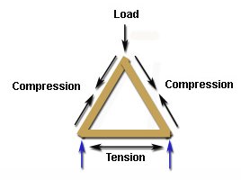

Which beam design makes the strongest truss?
As a continuation of the above suggestion, you could combine a couple of
trusses and see how they then react to the loads. After all, in the middle node
at the bottom, tension now becomes compression.
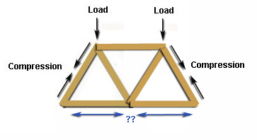

Radial and Harp cable-stayed bridges
I saw this interesting "structures" EEI at a Panel Meeting. It was undertaken by students at Redlands College, near Brisbane. My thanks to student Josh for use of his diagrams and to physics teacher Dan Graham for providing the details.
 |
 |
A harp bridge on the other hand, maintains a constant angle between the different cables and the pillar. |
A radial bridge has one anchoring point for all of its cables and the differences between the different cables are their angles with the pillar. |
Students investigated two types of cable-stayed bridges - radial and harp - for the relationship between the angle of the cable and the tension within it. They used a Pasco tension protractor to measure the tension in the string and the angle to the vertical. The analysis seems pretty obvious - is there a relationship between angle and tension for the stays as a function of increasing load on the deck.
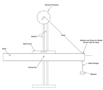 |
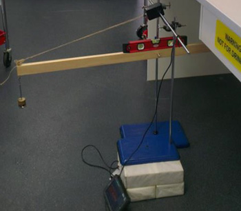 |
| Josh's diagram of the setup for his investigation - taken from his EEI with permission. Details (You Tube) on the Pasco tension protractor here. | As weights were added to the deck, the boss head was adjusted to keep the deck horizontal, and the angle and force recorded. |
How strong is silkworm silk?
Silk is a continuous filament fibre consisting of fibroin protein secreted
from glands in the head of each silkworm larva and a gum which cements the two
filaments together. To make useful thread for clothing, the raw silk is twisted
into a strand sufficiently strong for weaving or knitting. Four different types
of silk thread may be produced from this procedure: crepe, tram, thrown singles
and organzine. Crepe is made by twisting individual threads of raw silk,
doubling two or more of these together, and then twisting them again. Tram
is made by twisting two or more threads in only one direction. Thrown singles
are individual threads that are twisted in only one direction. Organzine
is a thread made by giving the raw silk a preliminary twist in one direction and
then twisting two of these threads together in the opposite direction. How does
the strength of the four methods compare? What's the hypothesis? You can get cocoons from ebay for $12 including postage for 33 cocoons. Posted from the Sunshine Coast, Queensland.

The effect of light on degradable materials
Biodegradable plastics are seen by many as a promising solution to the
problem of single-use conventional plastic bags. Although there are a variety of
degradable plastics which may assist reducing the resource wastage and litter
problems associated with plastic shopping bags, there is unfortunately no easy
solution. Degradability is the ability of materials to break down, by bacterial
(biodegradable), thermal (oxidative) or ultraviolet (photodegradable) action. If
you can get hold of a degradable plastic bag you could test the thermal and
photodegradable properties by measure the breaking strain before and after treatment. Is the wavelength
important, or is it just the intensity? Is temperature important, or just time?
A great EEI and so useful too, but I wonder if it would be more suitable for Chemistry. A source of biodegradabe plastic are the wrappers
some magazine come in (ask at the library or your teacher): these include Chemistry in Australia, Australian Physics and New Scientist (see photos below).


Polarisation of light in acidified sugar solution
Certain materials (sugar in this experiment) are optically active because
the molecules themselves have a twist in them. When linearly polarized light
passes through an optically active material, its direction of polarization is
rotated. The angle of rotation depends on the thickness of the material and the
wavelength of the light. You could make up a solution of sugar (sucrose) and
hydrolyse it using dilute acid. As the reaction proceeds, the degree of
polarisation changes and this can be observed using crossed polarisers either
side of the solution placed on an OHP. You could look at the effect of angle vs.
concentration vs time; depth effects; acidity effects; temperature.
Comparing the strength of laminated
and unlaminated wood beams
Make your own plywood out of paddlepop sticks. How does breaking force or
deflection vary with number of sticks? Turn the beam on it's side and try
again.
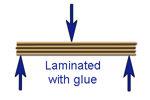
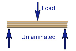
How do different woods expand when they are wet?
In which direction do they swell (if at all)? Is it a linear function with %
moisture? If they swell, do they become more or less dense? What physics
principles are being tested?
HERE ARE SOME WITHOUT HINTS
High static, low static and anti-static carpets
Why does cling wrapping cling?
The pitch of xylophone bars of different materials
What is the range limit for a string telephone?
The harmonics in a note, using Helmholtz resonators
Humidity and the speed of sound in air
The speed of sound in salt and fresh water
An efficient thermopile
Jacob's ladder
The Tesla coil
Vibration in a wire carrying AC electricity
Negative resistance phenomena
Practical uses of the Hall effect
Eddy current heating
Paramagnetism
Rainbows
Schlieren photography
Moiré fringes as measuring devices
Triboluminescence
Phosphenes
Holography
Producing a hologram
Thin-film interference
Kaleidoscopes
Anamorphic art
Tyndall figures
Tyndall scattering and the sunset
The Geissler tube
A Wilson cloud chamber
Celt stones
Skipping stones
The Marangoni effect
Leidenfrost phenomena
Lichtenberg figures
Fraunhofer patterns
The effect of cooling fins
Maxwell's spot
Kanizsa figures
The McCollough effect
The Pockels effect: or Pockels electro-optic effect, produces double refraction in certain crystals when a constant or varying electric field is applied.
Applications of the pantograph
 Go to New Century Senior Physics - Second Edition Home Page
 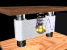 Return to Senior Physics
Resources Home Page
Return to Senior Physics
Resources Home Page